14.3: The Flux Control Coefficient

Search Fundamentals of Biochemistry

Introduction

Metabolic control analysis (MCA) is one method used to address the complexity of dynamic changes of species in a complex metabolic system. As such, an understanding of MCA would apply to complex signal transduction pathways as well as to other emerging areas in systems biology. In MCA, external inputs (source) and outputs (exits), and pools and reservoirs exist which are connected to the internal metabolic enzymes, reactants, and products of the pathway connecting the two external reservoirs.

In studying complex metabolic systems, what is interesting to know is not just the \(K_m\) or \(V_m\) of particular enzymes (such as those far from equilibrium or catalyzing “rate limiting” steps based on in vitro studies), but rather the control parameters, known as control coefficients, for the system. These coefficients are properties of the whole pathway as an emerging system with properties different from those of the individual steps. For another example of an emergent property, consider consciousness. It must emerge from the incredible assembly of around 90 billion neurons in the brain forming around 10¹⁵ synapses.  It cannot simply be predicted from the properties of isolated neurons. Three especially relevant parameters are used in metabolic control analyses, the Flux Control Coefficient, the Concentration Control Coefficient, and the Elasticity Coefficient

To understand how a pathway is regulated and how scientists modify it to meet their demands, one needs to understand these coefficients.  In particular, we would like to know which:

• parameters have the greatest effect (increase or decrease) on a preferred outcome;
• properties of the system make it most resilient or fragile;
• parameters should be measured most accurately

The Flux Control Coefficient

The Flux Control Coefficient (\(C_{Ei}^{J}\)) gives the relative fractional change in pathway flux \(J\) (\(dJ/J\)) (a system variable) with fractional change in concentration or activity of an enzyme \(Ei\) (\(du_i/u_i\)). The change in the concentration of an enzyme can arise from increased synthesis or degradation of the enzyme, a change in a modifier (an inhibitor or activator), a covalent modification, the presence of inhibitor RNA, mutations, etc. Again, the word flux \(J\) is used to describe the rate of the system whereas rate or velocity \(v\) is used to describe an individual enzyme in the system. Think of \(u\) as “units” of activity”.

The Flux Control Coefficient (\(C_{Ei}^{J}\)) can also be written as

\[C_{Ei}^{J}=\dfrac{d J}{d u} \dfrac{u}{J} \label{15} \]

The \(dJ/du\) in Equation \ref{15} suggests that the \(C_{Ei}^{J}\) is equal to the slope of a plot of \(J\) vs u multiplied by \(u/J\) at that point. Alternatively, it is the actual slope of an ln-ln plot of \(\ln J\) vs \(\ln u\). A more formal definition would be obtained using partial derivatives (a normal derivative like dy/dx with everyother variable held constant - in this case all other enzyme concentrations or activities other than the one under study :

\[C_{E i}^{J}=\dfrac{\dfrac{\partial J}{J}}{\dfrac{\partial u}{u}}=\dfrac{\partial \ln J}{\partial \ln u_{i}} \label{16} \]

\(C_{Ei}^{J}\) clearly shows how the system flux changes with changes in the activity of a single enzyme. The variable ui is a property of an enzyme (a local property) but J and concentrations (for the concentration coefficient – see below) are systems variables. Every enzyme in a pathway hence has a flux control coefficient. How are they related? It makes sense that the sum of all of the individual \(C_{Ei}^{J}=1\) as the fractional change in flux, \(∂J/J\), is equal in magnitude to the fractional change in all enzyme activities. This relationship, shown below, is called the Summation Theorem.

\[\sum_{i=1}^{n} C_{E i}^{J}=1 \label{17} \]

This equation would predict that if there were one magical enzyme X that was truly rate limiting and as such completely controlled that rate, then C^J_Ex = 1 for that enzyme and 0 for all the rest of the enzymes. Yet this is counterintuitive since if all the enzymes are linked their responses should also be linked. Hence the control of flux is shared by all enzymes.

Another way to think about this is to consider a linear set of connected reactions. For these enzymes, \(C_{Ei}^{J}\) would vary between 0 and 1. If one enzyme was completely rate limiting, its \(C_{Ei}^{J}\) would be 1 indicating that the fractional change in flux, \(∂J/J\), is equal to the fractional change in enzyme concentration (or activity) \(u\), \(∂u/u\), for enzyme X. This implies that all change in flux is accounted for by the change in the concentration of enzyme X. This is a bit difficult to believe so it would make sense to think of the control of a pathway as being distributed over all the enzymes in the pathway. Plots of flux \(J\) vs enzyme activity u are similar to rectangular hyperbolas. Hence the flux coefficient changes with enzyme activity and with flux so at different fluxes, different enzyme flux coefficients would change as well. “Control” gets redistributed in the pathway.

Textbooks often describe that ideally the first step of a linear pathway would be the committed step and be rate limiting. But think of this. If the end product of a pathway feeds back and inhibits the first enzyme in the pathway, then the last enzyme influences the first even though the last is not considered “rate limiting”. Now if another enzyme removes the last product and hence first enzyme's feedback inhibitor of the pathway, that enzyme determines flux as well. This again shows that flux control is distributed throughout the system. The classical “rate limiting” enzyme might still have the largest \(C_{Ei}^{J}\) of the pathways, but if the system is in a steady state, all enzymes have the same rate. Hence the term “rate-limiting” is a bit useless in a pathway. Analysis of flux control coefficients gives a truly quantitative analysis of the system pathway.

Phosphofructokinase is said to be a “key” enzyme in glycolysis as it is one of three enzymes in the pathway that is characterized by a large negative free energy difference.   Figure \(\PageIndex{1}\):

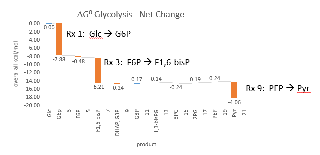
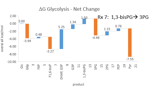
Figure \(\PageIndex{1}\): ΔG⁰ and ΔG values for enzymes in glycolysis

It is also highly regulated. However, Heinisch et al (Molecular and General Genetics, 202, 75-82) found that increasing its concentration 3.5 fold in fermenting yeast did not affect the flux of ethanol production.

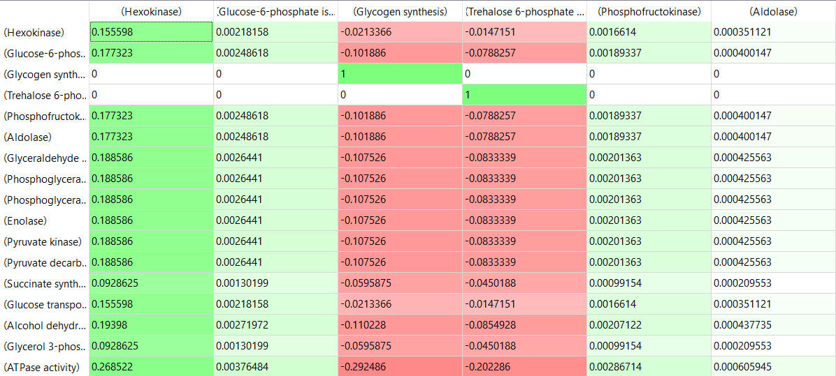
Here are some results of "sensitivity analyses" of yeast glycolysis showing the effect of small changes (up to 5%) on the flux control coefficients of glycolytic enzymes. The changes in the enzymes for these analyses are 1%. The numbers are scaled values that represent a relative change. A value of + 0.5 means that if the parameter is increased by 10%, the target value will increase by 5%. A column shows the rate of a reaction that is changed and the row indicates the flux of the reaction that has been affected. Green represents positive values and red negative with the intensity of the color correlating with the extent of the change. The table is split with column 1 of the first table applying to tables 2 and 3 as well.

Table, part 2, continued:

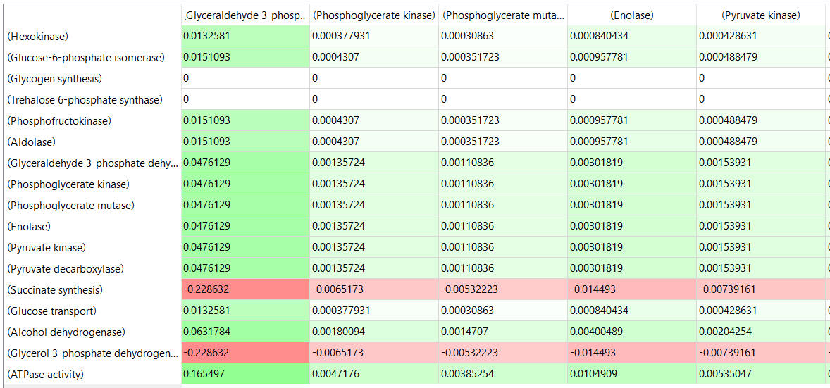
table, part 3, continued

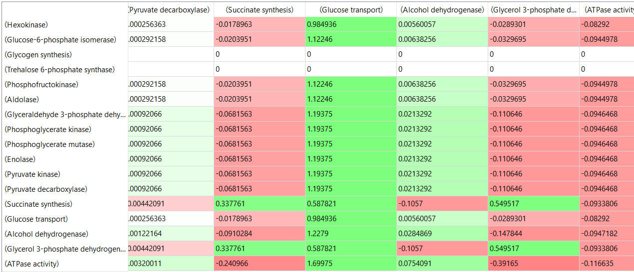
Some things to note:

• almost everything has changed in each column, which shows that a change in one enzyme affects all enzymes;
• 2 adjacent rows often have identical numbers since they describe two connected reactions (without branches) so their steady state fluxes will be the same;
• the sum of the C^J_Ei values across the same row in both tables is 1 (summation theorem);
• perturbations of the "big 3" enzymes for steps 1,3, and 10 in glycolysis (hexokinase, phosphofructokinase, and pyruvate kinase), all of which proceed with a significant -ΔG⁰ and -ΔG, have minor effects on the flux.

It should be clear from these results that you can't predict the enzymes that control the flux without this kind of mathematical analysis. Don't rely on just your "biochemical intuition"

Flux Control in Aerobic Glycolysis

Let's look at another pathway for which we can run a full simulation using Vcell - aerobic glycolysis.  We have mostly encountered glycolysis as a central anaerobic pathway in almost all organisms.  In some cases, it can also run aerobically.  One prime example is in cancer cells in which there is a need for energy in the form of ATP but also for anabolic building blocks so cells can proliferate - a hallmark of cancer cells.  Aerobic glycolysis was noted by Warbug and this effect now has his name.  

Aerobic glycolysis has been modeled in yeast cells.  The pathway is shown in Figure \(\PageIndex{2}\) below.  

Figure \(\PageIndex{2}\):  Schematic of the glycolysis model with chemical reactions and allosteric points of regulation described. Alexander A Shestov et al.  (2014) Quantitative determinants of aerobic glycolysis identify flux through the enzyme GAPDH as a limiting step. eLife 3:e03342.  https://doi.org/10.7554/eLife.03342.  Creative Commons Attribution License

Abbreviations: GLC—glucose, G6P—glucose-6-phosphate, F6P—fructose-6-phosphate, FBP—fructose-1,6,-bisphosphate, F26BP—fructose-2,6,-bisphosphate, GAP—glcyceraldehyde-3-phosphate, DHAP—dihydroxyacetone phosphate, BPG—1,3 bisphosphoglycerate, 3PG—3-phosphoglycerate, 2PG—2-phosphoglycerate, PEP—phosphoenolpyruvate, PYR—pyruvate, SER—Serine, GLY—glycine, Lac—lactate, MAL—malate, ASP—aspartate, Pi—inorganic phosphate, CI—creatine, PCI—phosphophocreatine, GTR—glucose transporter, HK—hexokinase, PGI—phosphoglucoisomerase, PFK—phosphofructokinase, ALD—aldolase, TPI—triosephosphoisomerase, GAPDH—glyceraldehyde-phosphate dehydrogenase, PGK—phosphoglycerate kinase, PGM—phosphoglycerate mutase, ENO—enolase, PK—pyruvate kinase, LDH—lactate dehydrogenase, MCT—monocarboxylate transporter, PDH—pyruvate dehydrogenase, CK—creatine kinase.  

The Warburg Effect W can be quantitatively described by the ratio of the flux of pyruvate to lactate (J_Lac) compared to the flux of pyruvate entry into the mitochondria and subsequent consumption of O₂  by mitochondrial oxidative phosphorylation (J_ox), so W = J_Lac/J_ox).  

Usually in normal conditions for healthy cells, W <0.10, which means that less than 10% of glucose is converted (or diverted) to lactate.  On average for different tissues, W < 0.3.  Hence some lactate is always being made.  High values of W (> 1) mean that most glucose is diverted to lactate synthesis. The W values is determined by lots of factors that determine the energy state of cells, including rates of glucose uptake, ATP hydrolysis, and biosynthesis, as well as the balance of cytoplasmic and mitochondrial NAD⁺/NADH, hence the redox state of the cell. Key to the balance leading to aerobic glycolysis is the need to reoxidize cytosolic NADH back to NAD⁺ under aerobic conditions so glycolysis can continue under conditions when there is a high growth rate.

How does a cell know which path to take, pyruvate to lactate (anaerobic), pyruvate to CO₂ with ATP synthesis (aerobic), or some of both?  In terms of metabolic control analysis, what controls the flux of pyruvate through these paths?  This is where computational modeling informed by experimental data helps. We can determine the flux control coefficient (\(C_{Ei}^{J}\)),  more easily written as FCC, for each enzyme in glycolysis to help us understand what controls the flux.  Figure \(\PageIndex{3}\) metaphorically describes these different paths. In a way, the flux of pyruvate through these 3 choices, anaerobic, aerobic, and both (as reflected by the Warburg effect W) is then perhaps the best example to use to discuss flux control since the readers are likely very familiar with the concept of anaerobic and aerobic metabolism and the "switch" between them when running short sprints vs marathons.

Figure \(\PageIndex{3}\): Fluxs of pyruvate through multiple paths

Now let's run the Vcell model for aerobic glycolysis in yeast. 

---

MODEL

AerobicGlycolysis

Quantitative determinants of aerobic glycolysis identify flux through the enzyme GAPDH as a limiting step. .Shestov AA, Liu X, Ser Z, Cluntun AA, Hung YP, Huang L, Kim D, Le A, Yellen G, Albeck JG, Locasale JW.  eLife , 7/ 2014 , Volume 3 , PubMed ID: 25009227.  Biomodel MODEL1504010000

 

Select Load [model name] below

 Select Start to begin the simulation.

Interactive Element

Select Plot to change Y axis min/max, then Reset and Play  |  Select Slider to change which constants are displayed |  Select About  for software information.

Move the sliders to change the constants and see changes in the displayed graph in real-time.

Time course model made using Virtual Cell (Vcell), The Center for Cell Analysis & Modeling, at UConn Health.  Funded by NIH/NIGMS (R24 GM137787); Web simulation software (miniSidewinder) from Bartholomew Jardine and Herbert M. Sauro, University of Washington.  Funded by NIH/NIGMS (RO1-GM123032-04)

---

 

Where did all the parameters in the model come from?  They are derived experimentally and the goal of modeling is to produce a computational model that is consistent with the experimental findings which are fed into the model. 

The result of the model suggests that the Warburg effect is determined by the growth rate of the cells as well as the activity of mitochondria. The model does not support the idea that aerobic glycolysis results as a balance between energy needs and new biosynthesis as cells proliferate. Rather, the cells that proliferate the most have the most active mitochondria and hence lower levels of lactate production.   Redox balance appears to be key in pushing cells toward lactate synthesis and aerobic glycolysis. 

A key step is catalyzed by glyceraldehyde-3-phosphate dehydrogenase (GAPDH), the glycolytic enzyme that separates the top and bottom halves of glycolysis. Experimental data shows that in fact, flux through this enzyme is rate-limiting with the levels of F1,6-BP also being very important. Some key steps that were thought to be rate-limited in fact had negative fluxes through them. Negative flux control coefficients were found and confirmed for several steps thought to be rate-limiting in glycolysis. 

The flux control coefficients, given by the formula

\begin{equation}
C_{E i}^J=\frac{\frac{\partial J}{J}}{\frac{\partial u}{u}}=\frac{\partial \ln J}{\partial \ln u_i}
\end{equation}

were calculated for each enzyme in the glycolytic pathway.  The authors of the study used this equation for the Flux Control Coefficient:  

\begin{equation}
F C C=\frac{d \ln \left[J_{L A C T}\right]}{d \ln \left[E_i\right]}
\end{equation}  

The fluxes were measured for lactate production by using ¹³C-labeled lactate to get the absolute concentration of lactate, and then measuring the fluxes by measuring the changes in ¹³C-lactate production with time. Using these data and the selective inhibition by small drugs of each step in glycolysis to effectively alter the "concentration/activity of the enzyme", the FCC of each enzyme could be calculated.  The results are shown in Figure \(\PageIndex{4}\) below.

Figure \(\PageIndex{4}\): (left) Box plots of flux control coefficient (FCC) for lactate production for each enzymatic step in glycolysis (FCC = dlnJ_lac/dln E_i) where J_lac is the rate of pyruvate conversion to lactate, and E_i is the i^th enzyme in glycolysis for each step of glycolysis. (right) Box plots of flux control coefficient (FCC) for lactate production for Oxygen consumption (OxPhos) and ATP consumption (ATP). Shestov et al., ibid

The left-hand side of Figure 4 shows that two of the key enzymes that are thermodynamically favored in glycolysis, PFK (phosphofructokinase) and HK (hexokinase), both driven by ATP hydrolysis, have essentially negative flux coefficients, so they are NOT key in driving flux toward lactate.  Only one enzyme, GAPDH, is characterized by a positive flux coefficient. (Remember we are talking about flux coefficients, not the Warburg effect factor W.)

Also important, as mentioned above, is the concentration of F1,6BP (FBP in the figure below).  The model and data show that high levels of FBP and associated higher concentrations of the reactants in the first half of glycolysis (denoted by ↑↑ and large font size), and a corresponding depletion of substrates in the bottom half (denoted by ↓↓) actually cause a bottleneck in glycolysis and inhibit flux through GADPH.  Hence GADPH determines the flux through glycolysis. This "bottleneck" is associated with the redox and energy states of the cell.   This outcomes are illustrated in Figure \(\PageIndex{1}\) below.

Figure \(\PageIndex{5}\):

Figure \(\PageIndex{5}\):  A unified model of aerobic glycolysis. Shestov et al., ibid

When there is a balance of metabolites in the top and bottom halves of glycolysis (right hand size), including both high levels in both top and bottom (denoted by ↑↑ and font size) or low levels in both (denoted by ↓↓ and font size), no bottleneck at GAPDH exists and flux through glycolysis is determined by the usual "suspects", hexokinase and phosphofructokinase.

The results described above are those predicted by computational modeling.  Do experimental data support the model?  The only way to know is to test the model.  This was done by using drugs to inhibit each of the enzymes in glycolysis.  This offers an effective way to change the "effective" concentration or activity in the enzyme.  From this data, flux changes due to changes at each step could be determined. These data supported the computation results - GADPH regulates aerobic metabolism in normal as well as.  When the top half substrates were elevated, the blockade of flux was determined by GADPH.  In Chapter 13, we studied all of the glycolytic enzymes and the myriad of small molecules that control the activity of the 3 major enzymes that have the biggest thermodynamic push, HK, PFK and PK.  GADPDH appears to be equally important.  It is known to be regulated by many mechanisms, including post-translational modifications, such as nitrosylation, and modification of its active site cysteine with ROS.  Perhaps this helps regulate the balance between anaerobic and aerobic glycolysis.  Also, there are high levels of expression of GADPH in cells engaged in aerobic glycolysis.