11.2: Foraging Ecology

Foraging

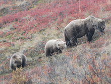
Grizzly bear (Ursus arctos horribilis) mother and cubs foraging in Denali National Park, Alaska.

Foraging is searching for wild food resources. It affects an animal's fitness because it plays an important role in an animal's ability to survive and reproduce.^[1] Foraging theory is a branch of behavioral ecology that studies the foraging behavior of animals in response to the environment where the animal lives.

Behavioral ecologists use economic models to understand foraging; many of these models are a type of optimal model. Thus foraging theory is discussed in terms of optimizing a payoff from a foraging decision. The payoff for many of these models is the amount of energy an animal receives per unit time, more specifically, the highest ratio of energetic gain to cost while foraging.^[2] Foraging theory predicts that the decisions that maximize energy per unit time and thus deliver the highest payoff will be selected for and persist. Key words used to describe foraging behavior include resources, the elements necessary for survival and reproduction which have a limited supply, predator, any organism that consumes others, prey, an organism that is eaten in part or whole by another,^[1] and patches, concentrations of resources.

Behavioral ecologists first tackled this topic in the 1960s and 1970s. Their goal was to quantify and formalize a set of models to test their null hypothesis that animals forage randomly. Important contributions to foraging theory have been made by:

• Eric Charnov, who developed the marginal value theorem to predict the behavior of foragers using patches;
• Sir John Krebs, with work on the optimal diet model in relation to tits and chickadees;
• John Goss-Custard, who first tested the optimal diet model against behavior in the field, using redshank, and then proceeded to an extensive study of foraging in the common pied oystercatcher

Factors influencing foraging behavior

A troop of olive baboons (Papio anubis) foraging in Laikipia, Kenya. Young primates learn from elders in their group about proper foraging.

Several factors affect an animal's ability to forage and acquire profitable resources.

Learning

Learning is defined as an adaptive change or modification of a behavior based on a previous experience.^[3] Since an animal's environment is constantly changing, the ability to adjust foraging behavior is essential for maximization of fitness. Studies in social insects have shown that there is a significant correlation between learning and foraging performance.^[3]

In nonhuman primates, young individuals learn foraging behavior from their peers and elders by watching other group members forage and by copying their behavior.^[4] Observing and learning from other members of the group ensure that the younger members of the group learn what is safe to eat and become proficient foragers.

One measure of learning is 'foraging innovation'—an animal consuming new food, or using a new foraging technique in response to their dynamic living environment.^[5] Foraging innovation is considered learning because it involves behavioral plasticity on the animal's part. The animal recognizes the need to come up with a new foraging strategy and introduce something it has never used before to maximize his or her fitness (survival). Forebrain size has been associated with learning behavior. Animals with larger brain sizes are expected to learn better.^[5] A higher ability to innovate has been linked to larger forebrain sizes in North American and British Isle birds according to Lefebvre et al. (1997).^[6] In this study, bird orders that contained individuals with larger forebrain sizes displayed a higher amount of foraging innovation. Examples of innovations recorded in birds include following tractors and eating frogs or other insects killed by it and using swaying trees to catch their prey.^[5]

Another measure of learning is spatio-temporal learning (also called time-place learning), which refers to an individual's ability to associate the time of an event with the place of that event.^[7] This type of learning has been documented in the foraging behaviors of individuals of the stingless bee species Trigona fulviventris.^[7] Studies showed that T. fulviventris individuals learned the locations and times of feeding events, and arrived to those locations up to thirty minutes before the feeding event in anticipation of the food reward.^[7]

Genetics

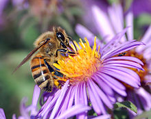
A European honey bee extracts nectar. According to Hunt (2007), two genes have been associated with the sugar concentration of the nectar honey bees collect.

Foraging behavior can also be influenced by genetics. The genes associated with foraging behavior have been widely studied in honeybees with reference to the following; onset of foraging behavior, task division between foragers and workers, and bias in foraging for either pollen or nectar.^[5][8] Honey bee foraging activity occurs both inside and outside the hive for either pollen or nectar. Similar behavior is seen in many social wasps, such as the species Apoica flavissima. Studies using quantitative trait loci (QTL) mapping have associated the following loci with the matched functions; Pln-1 and Pln-4 with onset of foraging age, Pln-1 and 2 with the size of the pollen loads collected by workers, and Pln-2 and pln-3 were shown to influence the sugar concentration of the nectar collected.^[8]

Predators and parasites

The presence of predators while a (prey) animal is foraging affects its behaviour. In general, foragers balance the risk of predation with their needs, thus deviating from the foraging behaviour that would be expected in the absence of predators.^[9]

Similarly, parasitism can affect the way in which animals forage. Parasitism can affect foraging at several levels. Animals might simply avoid food items that increase their risk of being parasitized, as when the prey items are intermediate hosts of parasites. Animals might also avoid areas that would expose them to a high risk of parasitism. Finally, animals might effectively self-medicate, either prophylactically or therapeutically.

Types of foraging

Foraging can be categorized into two main types. The first is solitary foraging, when animals forage by themselves. The second is group foraging.

Solitary foraging

Solitary foraging includes the variety of foraging in which animals find, capture and consume their prey alone. Individuals can manually exploit patches or they can use tools to exploit their prey. For example, Bolas spiders attack their prey by luring them with a scent identical to the female moth's sex pheromones.^[11] Animals may choose to forage on their own when the resources are abundant, which can occur when the habitat is rich or when the number of conspecifics foraging are few. In these cases there may be no need for group foraging.^[12] In addition, foraging alone can result in less interaction with other foragers, which can decrease the amount of competition and dominance interactions an animal deals with. It will also ensure that a solitary forager is less conspicuous to predators.^[13] Solitary foraging strategies characterize many of the phocids (the true seals) such as the elephant and harbor seals. An example of an exclusive solitary forager is the South American species of the harvester ant, Pogonomyrmex vermiculatus.^[14]

Solitary foraging and optimal foraging theory

The theory scientists use to understand solitary foraging is called optimal foraging theory (described in detail below). This theory argues that because of the key importance of successful foraging to an individual's survival, it should be possible to predict foraging behavior by using decision theory to determine the behavior that an "optimal forager" would exhibit. Such a forager has perfect knowledge of what to do to maximize usable food intake. While the behavior of real animals inevitably departs from that of the optimal forager, optimal foraging theory has proved very useful in developing hypotheses for describing real foraging behavior. Departures from optimality often help to identify constraints either in the animal's behavioral or cognitive repertoire, or in the environment, that had not previously been suspected. With those constraints identified, foraging behavior often does approach the optimal pattern even if it is not identical to it. In other words, we know from optimal foraging theory that animals are not foraging randomly even if their behavior doesn't perfectly match what is predicted by OFT.

Group foraging

Group foraging is when animals find, capture and consume prey in the presence of other individuals. In other words, it is foraging when success depends not only on your own foraging behaviors but the behaviors of others as well.^[20] An important note here is that group foraging can emerge in two types of situations. The first situation is frequently thought of and occurs when foraging in a group is beneficial and brings greater rewards known as an aggregation economy.[1] The second situation occurs when a group of animals forage together but it may not be in an animal's best interest to do so known as a dispersion economy. Think of a cardinal at a bird feeder for the dispersion economy. We might see a group of birds foraging at that bird feeder but it is not in the best interest of the cardinal for any of the other birds to be there too. The amount of food the cardinal can get from that bird feeder depends on how much it can take from the bird feeder but also depends on how much the other birds take as well.

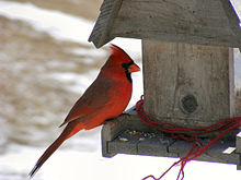
A male northern cardinal at a bird feeder. Birds feeding at a bird feeder is an example of a dispersion economy. This is when it may not be in an animal's best interest to forage in a group.

In red harvester ants, the foraging process is divided between three different types of workers: nest patrollers, trail patrollers, and foragers. These workers can utilize many different methods of communicating while foraging in a group, such as guiding flights, scent paths, and "jostling runs", as seen in the eusocial bee Melipona scutellaris.^[21]

Chimpanzees in the Taï Forest in Côte d'Ivoire also engage in foraging for meats when they can, which is achieved through group foraging. Positive correlation has been observed between the success of the hunt and the size of the foraging group. The chimps have also been observed implying rules with their foraging, where there is a benefit to becoming involved through allowing successful hunters first access to their kills.^[22][23][24]

Cost and benefits of group foraging

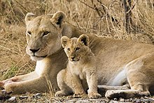
Female lions make foraging decisions and more specifically decisions about hunting group size with protection of their cubs and territory defense in mind.^[25]

As already mentioned, group foraging brings both costs and benefits to the members of that group. Some of the benefits of group foraging include being able to capture larger prey,^[25] being able to create aggregations of prey,^[26] being able to capture prey that are difficult or dangerous and most importantly reduction of predation threat.^[20] With regard to costs, however, group foraging results in competition for available resources by other group members. Competition for resources can be characterized by either scramble competition whereby each individual strives to get a portion of the shared resource, or by interference competition whereby the presence of competitors prevents a forager's accessibility to resources.^[1] Group foraging can thus reduce an animal's foraging payoff.^[20]

Group foraging may be influenced by the size of a group. In some species like lions and wild dogs, foraging success increases with an increase in group size then declines once the optimal size is exceeded. A myriad number of factors affect the group sizes in different species. For example, lionesses (female lions) do not make decisions about foraging in a vacuum. They make decisions that reflect a balance between obtaining food, defending their territory and protecting their young. In fact, we see that lion foraging behavior does not maximize their energy gain. They are not behaving optimally with respect to foraging because they have to defend their territory and protect young so they hunt in small groups to reduce the risk of being caught alone.^[25] Another factor that may influence group size is the cost of hunting. To understand the behavior of wild dogs and the average group size we must incorporate the distance the dogs run.^[27]

Group foraging and the ideal free distribution

The theory scientists use to understand group foraging is called the Ideal free distribution. This is the null model for thinking about what would draw animals into groups to forage and how they would behave in the process. This model predicts that animals will make an instantaneous decision about where to forage based on the quality (prey availability) of the patches available at that time and will choose the most profitable patch, the one that maximizes their energy intake. This quality depends on the starting quality of the patch and the number of predators already there consuming the prey.

Video

 

BIO 270 Material: Optimal foraging theory

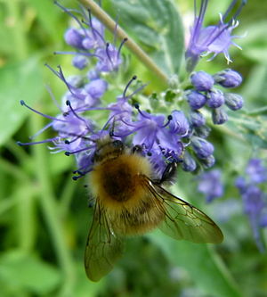
Worker bees forage nectar not only for themselves, but for their whole hive community. Optimal foraging theory predicts that this bee will forage in a way that will maximize its hive's net yield of energy.

Optimal foraging theory (OFT) is a behavioral ecology model that helps predict how an animal behaves when searching for food. Although obtaining food provides the animal with energy, searching for and capturing the food require both energy and time. To maximize fitness, an animal adopts a foraging strategy that provides the most benefit (energy) for the lowest cost, maximizing the net energy gained. OFT helps predict the best strategy that an animal can use to achieve this goal.

OFT is an ecological application of the optimality model. This theory assumes that the most economically advantageous foraging pattern will be selected for in a species through natural selection.^[29] When using OFT to model foraging behavior, organisms are said to be maximizing a variable known as the currency, such as the most food per unit time. In addition, the constraints of the environment are other variables that must be considered. Constraints are defined as factors that can limit the forager's ability to maximize the currency. The optimal decision rule, or the organism's best foraging strategy, is defined as the decision that maximizes the currency under the constraints of the environment. Identifying the optimal decision rule is the primary goal of the OFT.^[30]

Building an optimal foraging model

An optimal foraging model generates quantitative predictions of how animals maximize their fitness while they forage. The model building process involves identifying the currency, constraints, and appropriate decision rule for the forager.^[30][31]

Currency is defined as the unit that is optimized by the animal. It is also a hypothesis of the costs and benefits that are imposed on that animal.^[32] For example, a certain forager gains energy from food, but incurs the cost of searching for the food: the time and energy spent searching could have been used instead on other endeavors, such as finding mates or protecting young. It would be in the animal's best interest to maximize its benefits at the lowest cost. Thus, the currency in this situation could be defined as net energy gain per unit time.^[30] However, for a different forager, the time it takes to digest the food after eating could be a more significant cost than the time and energy spent looking for food. In this case, the currency could be defined as net energy gain per digestive turnover time instead of net energy gain per unit time.^[33] Furthermore, benefits and costs can depend on a forager's community. For example, a forager living in a hive would most likely forage in a manner that would maximize efficiency for its colony rather than itself.^[32] By identifying the currency, one can construct a hypothesis about which benefits and costs are important to the forager in question.

Constraints are hypotheses about the limitations that are placed on an animal.^[32] These limitations can be due to features of the environment or the physiology of the animal and could limit their foraging efficiency. The time that it takes for the forager to travel from the nesting site to the foraging site is an example of a constraint. The maximum number of food items a forager is able to carry back to its nesting site is another example of a constraint. There could also be cognitive constraints on animals, such as limits to learning and memory.^[30] The more constraints that one is able to identify in a given system, the more predictive power the model will have.^[32]

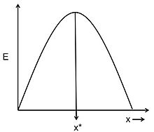
Figure 1. Energy gain per cost (E) for adopting foraging strategy x. Adapted from Parker & Smith.^[34]

Given the hypotheses about the currency and the constraints, the optimal decision rule is the model's prediction of what the animal's best foraging strategy should be.^[30] Possible examples of optimal decision rules could be the optimal number of food items that an animal should carry back to its nesting site or the optimal size of a food item that an animal should feed on. Figure 1, shows an example of how an optimal decision rule could be determined from a graphical model.^[34] The curve represents the energy gain per cost (E) for adopting foraging strategy x. Energy gain per cost is the currency being optimized. The constraints of the system determine the shape of this curve. The optimal decision rule (x*) is the strategy for which the currency, energy gain per costs, is the greatest. Optimal foraging models can look very different and become very complex, depending on the nature of the currency and the number of constraints considered. However, the general principles of currency, constraints, and optimal decision rule remain the same for all models.

To test a model, one can compare the predicted strategy to the animal's actual foraging behavior. If the model fits the observed data well, then the hypotheses about the currency and constraints are supported. If the model doesn't fit the data well, then it is possible that either the currency or a particular constraint has been incorrectly identified.^[32]

Different feeding systems and classes of predators

Optimal foraging theory is widely applicable to feeding systems throughout the animal kingdom. Under the OFT, any organism of interest can be viewed as a predator that forages prey. There are different classes of predators that organisms fall into and each class has distinct foraging and predation strategies.

• True predators attack large numbers of prey throughout their life. They kill their prey either immediately or shortly after the attack. They may eat all or only part of their prey. True predators include tigers, lions, whales, sharks, seed-eating birds, ants.^[35]
• Grazers eat only a portion of their prey. They harm the prey, but rarely kill it. Grazers include antelope, cattle, and mosquitoes.
• Parasites, like grazers, eat only a part of their prey (host), but rarely the entire organism. They spend all or large portions of their life cycle living in/on a single host. This intimate relationship is typical of tapeworms, liver flukes, and plant parasites, such as the potato blight.
• Parasitoids are mainly typical of wasps (order Hymenoptera), and some flies (order Diptera). Eggs are laid inside the larvae of other arthropods which hatch and consume the host from the inside, killing it. This unusual predator–host relationship is typical of about 10% of all insects.^[36] Many viruses that attack single-celled organisms (such as bacteriophages) are also parasitoids; they reproduce inside a single host that is inevitably killed by the association.

The optimization of these different foraging and predation strategies can be explained by the optimal foraging theory. In each case, there are costs, benefits, and limitations that ultimately determine the optimal decision rule that the predator should follow.

The optimal diet model

One classical version of the optimal foraging theory is the optimal diet model, which is also known as the prey choice model or the contingency model. In this model, the predator encounters different prey items and decides whether to eat what it has or search for a more profitable prey item. The model predicts that foragers should ignore low profitability prey items when more profitable items are present and abundant.^[37]

The profitability of a prey item is dependent on several ecological variables. E is the amount of energy (calories) that a prey item provides the predator. Handling time (h) is the amount of time it takes the predator to handle the food, beginning from the time the predator finds the prey item to the time the prey item is eaten. The profitability of a prey item is then defined as E/h. Additionally, search time (S) is the amount of time it takes the predator to find a prey item and is dependent on the abundance of the food and the ease of locating it.^[30] In this model, the currency is energy intake per unit time and the constraints include the actual values of E, h, and S, as well as the fact that prey items are encountered sequentially.

Model of choice between big and small prey

Using these variables, the optimal diet model can predict how predators choose between two prey types: big prey1 with energy value E1 and handling time h1, and small prey2 with energy value E2 and handling time h2. In order to maximize its overall rate of energy gain, a predator must consider the profitability of the two prey types. If it is assumed that big prey1 is more profitable than small prey2, then E1/h1 > E2/h2. Thus, if the predator encounters prey1, it should always choose to eat it, because of its higher profitability. It should never bother to go searching for prey2. However, if the animal encounters prey2, it should reject it to look for a more profitable prey1, unless the time it would take to find prey1 is too long and costly for it to be worth it. Thus, the animal should eat prey2 only if E2/h2 > E1/(h1+S1), where S1 is the search time for prey1. Since it is always favorable to choose to eat prey1, the choice to eat prey1 is not dependent on the abundance of prey2. But since the length of S1 (i.e. how difficult it is to find prey1) is logically dependent on the density of prey1, the choice to eat prey2 is dependent on the abundance of prey1.^[32]

Generalist and specialist diets

The optimal diet model also predicts that different types of animals should adopt different diets based on variations in search time. This idea is an extension of the model of prey choice that was discussed above. The equation, E2/h2 > E1/(h1+S1), can be rearranged to give: S1 > [(E1h2)/E2] – h1. This rearranged form gives the threshold for how long S1 must be for an animal to choose to eat both prey1 and prey2.^[32] Animals that have S1's that reach the threshold are defined as generalists. In nature, generalists include a wide range of prey items in their diet.^[38] An example of a generalist is a mouse, which consumes a large variety of seeds, grains, and nuts.^[39] In contrast, predators with relatively short S1's are still better off choosing to eat only prey1. These types of animals are defined as specialists and have very exclusive diets in nature.^[38] An example of a specialist is the koala, which solely consumes eucalyptus leaves.^[40] In general, different animals across the four functional classes of predators exhibit strategies ranging across a continuum between being a generalist and a specialist. Additionally, since the choice to eat prey2 is dependent on the abundance of prey1 (as discussed earlier), if prey1 becomes so scarce that S1 reaches the threshold, then the animal should switch from exclusively eating prey1 to eating both prey1 and prey2.^[32] In other words, if the food within a specialist's diet becomes very scarce, a specialist can sometimes switch to being a generalist.

Functional response curves

As previously mentioned, the amount of time it takes to search for a prey item depends on the density of the prey. Functional response curves show the rate of prey capture as a function of food density and can be used in conjunction with the optimal diet theory to predict foraging behavior of predators. There are three different types of functional response curves.^[41]

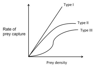
Figure 2. Three types of functional response curves. Adapted from Staddon.^[41]

For a Type I functional response curve, the rate of prey capture increases linearly with food density. At low prey densities, the search time is long. Since the predator spends most of its time searching, it eats every prey item it finds. As prey density increases, the predator is able to capture the prey faster and faster. At a certain point, the rate of prey capture is so high, that the predator doesn't have to eat every prey item it encounters. After this point, the predator should choose only the prey items with the highest E/h.^[42]

For a Type II functional response curve, the rate of prey capture negatively accelerates as it increases with food density.^[41] This is because it assumes that the predator is limited by its capacity to process food. In other words, as the food density increases, handling time increases. At the beginning of the curve, rate of prey capture increases nearly linearly with prey density and there is almost no handling time. As prey density increases, the predator spends less and less time searching for prey and more and more time handling the prey. The rate of prey capture increases less and less, until it finally plateaus. The high number of prey basically "swamps" the predator.^[42]

A Type III functional response curve is a sigmoid curve. The rate of prey capture increases at first with prey density at a positively accelerated rate, but then at high densities changes to the negatively accelerated form, similar to that of the Type II curve.^[41] At high prey densities (the top of the curve), each new prey item is caught almost immediately. The predator is able to be choosy and doesn't eat every item it finds. So, assuming that there are two prey types with different profitabilities that are both at high abundance, the predator will choose the item with the higher E/h. However, at low prey densities (the bottom of the curve) the rate of prey capture increases faster than linearly. This means that as the predator feeds and the prey type with the higher E/h becomes less abundant, the predator will start to switch its preference to the prey type with the lower E/h, because that type will be relatively more abundant. This phenomenon is known as prey switching.^[41]

Predator–prey interaction

Predator–prey coevolution often makes it unfavorable for a predator to consume certain prey items, since many anti-predator defenses increase handling time.^[43] Examples include porcupine quills, the palatability and digestibility of the poison dart frog, crypsis, and other predator avoidance behaviors. In addition, because toxins may be present in many prey types, predators include a lot of variability in their diets to prevent any one toxin from reaching dangerous levels. Thus, it is possible that an approach focusing only on energy intake may not fully explain an animal's foraging behavior in these situations.

The marginal value theorem and optimal foraging

The marginal value theorem is a type of optimality model that is often applied to optimal foraging. This theorem is used to describe a situation in which an organism searching for food in a patch must decide when it is economically favorable to leave. While the animal is within a patch, it experiences the law of diminishing returns, where it becomes harder and harder to find prey as time goes on. This may be because the prey is being depleted, the prey begins to take evasive action and becomes harder to catch, or the predator starts crossing its own path more as it searches.^[32] This law of diminishing returns can be shown as a curve of energy gain per time spent in a patch (Figure 3). The curve starts off with a steep slope and gradually levels off as prey becomes harder to find. Another important cost to consider is the traveling time between different patches and the nesting site. An animal loses foraging time while it travels and expends energy through its locomotion.^[30]

In this model, the currency being optimized is usually net energy gain per unit time. The constraints are the travel time and the shape of the curve of diminishing returns. Graphically, the currency (net energy gain per unit time) is given by the slope of a diagonal line that starts at the beginning of traveling time and intersects the curve of diminishing returns (Figure 3). In order to maximize the currency, one wants the line with the greatest slope that still touches the curve (the tangent line). The place that this line touches the curve provides the optimal decision rule of the amount of time that the animal should spend in a patch before leaving.

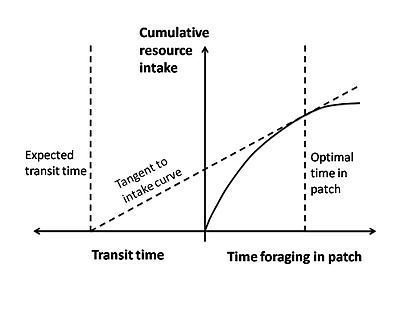
Figure 3. Marginal value theorem shown graphically.

Examples of optimal foraging models in animals

Figure 4. Right-shifted mussel profitability curve. Adapted from Meire & Ervynck.^[44]

Optimal foraging of oystercatchers

Oystercatcher mussel feeding provides an example of how the optimal diet model can be utilized. Oystercatchers forage on mussels and crack them open with their bills. The constraints on these birds are the characteristics of the different mussel sizes. While large mussels provide more energy than small mussels, large mussels are harder to crack open due to their thicker shells. This means that while large mussels have a higher energy content (E), they also have a longer handling time (h). The profitability of any mussel is calculated as E/h. The oystercatchers must decide which mussel size will provide enough nutrition to outweigh the cost and energy required to open it.[2] In their study, Meire and Ervynck tried to model this decision by graphing the relative profitabilities of different sized mussels. They came up with a bell-shaped curve, indicating that moderately sized mussels were the most profitable. However, they observed that if an oystercatcher rejected too many small mussels, the time it took to search for the next suitable mussel greatly increased. This observation shifted their bell-curve to the right (Figure 4). However, while this model predicted that oystercatchers should prefer mussels of 50–55 mm, the observed data showed that oystercatchers actually prefer mussels of 30–45 mm. Meire and Ervynk then realized the preference of mussel size did not depend only on the profitability of the prey, but also on the prey density. After this was accounted for, they found a good agreement between the model's prediction and the observed data.^[44]

Optimal foraging in starlings

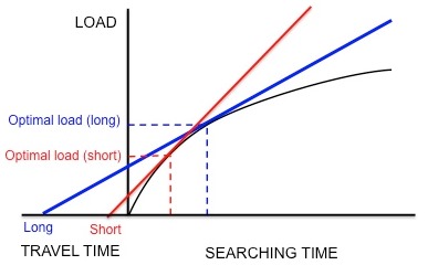
Figure 5. If starlings are maximizing net rate of energy gain, longer traveling time results in larger optimum load. Adapted from Krebs and Davies.^[32]

The foraging behavior of the European starling, Sturnus vulgaris, provides an example of how marginal value theorem is used to model optimal foraging. Starlings leave their nests and travel to food patches in search for larval leatherjackets to bring back to their young. The starlings must determine the optimal number of prey items to take back in one trip (i.e. the optimal load size). While the starlings forage within a patch, they experience diminishing returns: the starling is able to hold only so many leatherjackets in its bill, so the speed with which the parent picks up larvae decreases with the number of larvae that it already has in its bill. Thus, the constraints are the shape of the curve of diminishing returns and the travel time (the time it takes to make a round trip from the nest to a patch and back). In addition, the currency is hypothesized to be net energy gain per unit time.^[32] Using this currency and the constraints, the optimal load can be predicted by drawing a line tangent to the curve of diminishing returns, as discussed previously (Figure 3).

Kacelnik et al. wanted to determine if this species does indeed optimize net energy gain per unit time as hypothesized.^[45] They designed an experiment in which the starlings were trained to collect mealworms from an artificial feeder at different distances from the nest. The researchers artificially generated a fixed curve of diminishing returns for the birds by dropping mealworms at successively longer and longer intervals. The birds continued to collect mealworms as they were presented, until they reached an "optimal" load and flew home. As Figure 5 shows, if the starlings were maximizing net energy gain per unit time, a short travel time would predict a small optimal load and a long travel time would predict a larger optimal load. In agreement with these predictions, Kacelnik found that the longer the distance between the nest and the artificial feeder, the larger the load size. In addition, the observed load sizes quantitatively corresponded very closely to the model's predictions. Other models based on different currencies, such as energy gained per energy spent (i.e. energy efficiency), failed to predict the observed load sizes as accurately. Thus, Kacelnik concluded that starlings maximize net energy gain per unit time. This conclusion was not disproved in later experiments.^[46][47]

Video

 

References (Part 1)

References

1. Danchin, E.; Giraldeau, L. & Cezilly, F. (2008). Behavioural Ecology. New York: Oxford University Press. ISBN 978-0-19-920629-2.[page needed]
2. Hughes, Roger N, ed. (1989), Behavioural Mechanisms of Food Selection, London & New York: Springer-Verlag, p. v, ISBN 978-0-387-51762-9
3. Raine, N.E.; Chittka, L. (2008). "The correlation of learning speed and natural foraging success in bumble-bees'". Proceedings of the Royal Society B: Biological Sciences. 275 (1636): 803–08. doi:10.1098/rspb.2007.1652. PMC 2596909. PMID 18198141.
4. Rapaport, L.G.; Brown, G.R. (2008). "Social influences on foraging behavior in young nonhuman primates:learning what, where and how to eat". Evolutionary Anthropology: Issues, News, and Reviews. 17 (4): 189–201. doi:10.1002/evan.20180. S2CID 86010867.
5. Dugatkin, Lee Ann (2004). Principles of Animal Behavior.
6. Lefebvre, Louis; Patrick Whittle; Evan Lascaris; Adam Finkelstein (1997). "Feeding innovations and forebrain size in birds". Animal Behaviour. 53 (3): 549–60. doi:10.1006/anbe.1996.0330. S2CID 53146859.
7. Murphy, Christina M.; Breed, Michael D. (2008-04-01). "Time-Place Learning in a Neotropical Stingless Bee, Trigona fulviventris Guérin (Hymenoptera: Apidae)". Journal of the Kansas Entomological Society. 81 (1): 73–76. doi:10.2317/JKES-704.23.1. ISSN 0022-8567. S2CID 86256384.
8. Hunt, G.J.; et al. (2007). "Behavioral genomics of honeybee foraging and nest defense". Naturwissenschaften. 94 (4): 247–67. doi:10.1007/s00114-006-0183-1. PMC 1829419. PMID 17171388.
9. de Belle, J.S.; Hiliker, A.J.; Sokolowski, M.B. (1 September 1989). "Genetic localization of foraging (for): a major gene for larval behavior in Drosophila melanogaster". Genetics Society of America. 123 (1): 157–163. doi:10.1093/genetics/123.1.157 – via Oxford Academic.
10. Pereira, H S; MacDonald, D E; Hilliker, A J; Sokolowski, M B (1995-09-01). "Chaser (Csr), a new gene affecting larval foraging behavior in Drosophila melanogaster". Genetics. 141 (1): 263–270. doi:10.1093/genetics/141.1.263. ISSN 1943-2631.
11. de Belle, J.S.; Hiliker, A.J.; Sokolowski, M.B. (1 September 1989). "Genetic localization of foraging (for): a major gene for larval behavior in Drosophila melanogaster". Genetics Society of America. 123 (1): 157–163. doi:10.1093/genetics/123.1.157 – via Oxford Academic.
12. Roch, S.; von Ammon, L.; Geist, J.; Brinker, A. (2018). "Foraging habits of invasive three-spined sticklebacks ( Gasterosteus aculeatus ) – impacts on fisheries yield in Upper Lake Constance". Fisheries Research. 204: 172–80. doi:10.1016/j.fishres.2018.02.014.
13. Cruz-Rivera, Edwin; Hay, Mark E. (2000-01-01). "Can quantity replace quality? food choice, compensatory feeding, and fitness of marine mesograzers". Ecology. 81 (1): 201–19. doi:10.1890/0012-9658(2000)081[0201:CQRQFC]2.0.CO;2.
14. Hutchings, Michael R.; Athanasiadou, Spiridoula; Kyriazakis, Ilias; Gordon, Iain J. (11 August 2008). "Can animals use foraging behaviour to combat parasites?". Proceedings of the Nutrition Society. 62 (2): 361–370. doi:10.1079/PNS2003243. ISSN 1475-2719.
15. Hutchings, Michael R.; Judge, Johanna; Gordon, Iain J.; Athanasiadou, Spiridoula; Kyriazakis, Ilias (2006). "Use of trade-off theory to advance understanding of herbivore–parasite interactions". Mammal Review. 36 (1): 1–16. doi:10.1111/j.1365-2907.2006.00080.x. ISSN 1365-2907.
16. Hutchings, Michael R.; Athanasiadou, Spiridoula; Kyriazakis, Ilias; Gordon, Iain J. (11 August 2008). "Can animals use foraging behaviour to combat parasites?". Proceedings of the Nutrition Society. 62 (2): 361–370. doi:10.1079/PNS2003243. ISSN 1475-2719.
17. "Foraging Strategies | Encyclopedia.com". www.encyclopedia.com. Retrieved 2021-09-26.
18. Riedman, Marianne (1990). The pinnipeds: seals, sea lions, and walruses. Berkeley: University of California Press. ISBN 978-0-520-06497-3. ISBN The pinnipeds: seals, sea lions, and walruses By Marianne Riedman 1990.
19. le Roux, Aliza; Michael I. Cherry; Lorenz Gygax (5 May 2009). "Vigilance behaviour and fitness consequences: comparing a solitary foraging and an obligate group-foraging mammal". Behavioral Ecology and Sociobiology. 63 (8): 1097–1107. doi:10.1007/s00265-009-0762-1. S2CID 21961356.
20. Torres-Contreras, Hugo; Ruby Olivares-Donoso; Hermann M. Niemeyer (2007). "Solitary Foraging in the Ancestral South American Ant, Pogonomyrmex vermiculatus. Is it Due to Constraints in the Production or Perception of Trail Pheromones?". Journal of Chemical Ecology. 33 (2): 435–40. doi:10.1007/s10886-006-9240-7. PMID 17187299. S2CID 23930353.
21. O'Brien, W.J.; Browman, H.I.; Evans, B.I. (1990). "Search Strategies of Foraging Animals" (PDF). American Scientist. 78 (2): 152–160.
22. O'Brien, W.J.; Browman, H.I.; Evans, B.I. (1990). "Search Strategies of Foraging Animals" (PDF). American Scientist. 78 (2): 152–160.
23. Patterson, E.M.; Mann, J. (2011). "The Ecological Conditions That Favor Tool Use and Innovation in Wild Bottlenose Dolphins (Tursiops sp.)". PLOS ONE. 6 (7): e22243. doi:10.1371/journal.pone.0022243. PMC 3140497. PMID 21799801.
24. Rutz, C.; et al. (2010). "The ecological significance of tool use in New Caledonian Crows". Science. 329 (5998): 1523–26. doi:10.1126/science.1192053. PMID 20847272. S2CID 8888382.
25. Goodall, Jane (1964). "Tool-using and aimed throwing in a community of free-living chimpanzees". Nature. 201 (4926): 1264–66. doi:10.1038/2011264a0. PMID 14151401. S2CID 7967438.
26. MacArthur RH, Pianka ER (1966), "On the optimal use of a patchy environment.", American Naturalist, 100 (916): 603–09, doi:10.1086/282454, JSTOR 2459298, S2CID 86675558
27. Emlen, J. M. (1966), "The role of time and energy in food preference", The American Naturalist, 100 (916): 611–17, doi:10.1086/282455, JSTOR 2459299, S2CID 85723900
28. Stephens, D.W.; Brown, J.S. & Ydenberg, R.C. (2007). Foraging: Behavior and Ecology. Chicago: University of Chicago Press.[page needed][ISBN missing]
29. Hrncir, Michael; Jarau, Stefan; Zucchi, Ronaldo; Barth, Friedrich G. (2000). "Recruitment behavior in stingless bees, Melipona scutellaris and M. quadrifasciata . II. Possible mechanisms of communication" (PDF). Apidologie. 31 (1): 93–113. doi:10.1051/apido:2000109.
30. Boesch, C (1994). "Cooperative hunting in wild Chimpanzees". Animal Behaviour. 48 (3): 653–67. doi:10.1006/anbe.1994.1285. S2CID 53177700.
31. 1. Gomes 2. Boesch, 1. C M 2. C (2009). "Wild chimpanzees exchange meat for sex on a long term basis". PLOS ONE. 4 (4): e5116. doi:10.1371/journal.pone.0005116. PMC 2663035. PMID 19352509.
32. 1 Gomes 2 Boesch, 1 CM 2 C (2011). "Reciprocity and trades in wild west African chimpanzees". Behavioral Ecology and Sociobiology. 65 (11): 2183–96. doi:10.1007/s00265-011-1227-x. S2CID 37432514.
33. Packer, C.; Scheel, D.; Pusey, A.E. (1990). "Why lions form groups: food is not enough". American Naturalist. 136: 1–19. doi:10.1086/285079. S2CID 85145653.
34. Benoit-Bird, Kelly; Whitlow W. L. Au (January 2009). "Cooperative prey herding by the pelagic dolphin, Stenella longirostris" (PDF). The Journal of the Acoustical Society of America. 125 (1): 125–37. doi:10.1121/1.2967480. PMID 19173400. Archived from the original (PDF) on 2012-04-25. Retrieved 2011-11-29.
35. Creel, S; Creel N M (1995). "Communal hunting and pack size in African wild dogs, Lycaon pictus". Animal Behaviour. 50 (5): 1325–39. doi:10.1016/0003-3472(95)80048-4. S2CID 53180378.
36. BS Blades – Aurignacian Lithic Economy: Ecological Perspectives from Southwestern France Springer, 31 January 2001 Retrieved 2012-07-08 ISBN 0306463342
37. Ahrens, Robert N. M.; Walters, Carl J.; Christensen, Villy (2012). "Foraging arena theory". Fish and Fisheries. 13 (1): 41–59. doi:10.1111/j.1467-2979.2011.00432.x. ISSN 1467-2979.
38. Tupper, Mark; Juanes, Francis (2017-02-01). "Testing foraging arena theory: The effects of conspecific density and habitat type on time and energy budgets of juvenile cunner". Journal of Experimental Marine Biology and Ecology. 487: 86–93. doi:10.1016/j.jembe.2016.12.001. ISSN 0022-0981.
39. Stephens, D.W. (6 August 2008). "Optimal Foraging Theory". Encyclopedia of ecology. Elsevier: 2561–2566 – via ScienceDirect.

---

References (Part 2)

1. Werner, E. E.; Hall, D. J. (1974). "Optimal Foraging and the Size Selection of Prey by the Bluegill Sunfish (Lepomis macrochirus)". Ecology. 55 (5): 1042. doi:10.2307/1940354. JSTOR 1940354.
2. Sinervo, Barry (1997). "Optimal Foraging Theory: Constraints and Cognitive Processes" Archived 23 November 2015 at the Wayback Machine, pp. 105–130 in Behavioral Ecology. University of California, Santa Cruz.
3. Stephens, D. W. and Krebs, J. R. (1986) "Foraging Theory". 1st ed. Monographs in Behavior and Ecology. Princeton University Press. ISBN 9780691084428.[page needed]
4. Krebs, J. R. and Davies, N. B. (1989) An Introduction to Behavioral Ecology. 4th ed. Oxford: Blackwell Scientific Publications.[ISBN missing][page needed]
5. Verlinden, C.; Wiley, R. H. (1989). "The constraints of digestive rate: An alternative model of diet selection". Evolutionary Ecology. 3 (3): 264. doi:10.1007/BF02270727. S2CID 46608348.
6. Parker, G. A.; Smith, J. M. (1990). "Optimality theory in evolutionary biology". Nature. 348 (6296): 27. Bibcode:1990Natur.348...27P. doi:10.1038/348027a0.
7. Cortés, E.; Gruber, S. H.; Cortes, E. (1990). "Diet, Feeding Habits and Estimates of Daily Ration of Young Lemon Sharks, Negaprion brevirostris (Poey)". Copeia. 1990 (1): 204–218. doi:10.2307/1445836. JSTOR 1445836.
8. Godfray, H. C. J. (1994) Parasitoids: Behavioral and Evolutionary Ecology. Princeton University Press, Princeton.[ISBN missing][page needed]
9. Stephens, D.W., Brown, J.S., and Ydenberg, R.C. (2007). Foraging: Behavior and Ecology. Chicago: University of Chicago Press.[ISBN missing][page needed]
10. Pulliam, H. Ronald (1974). "On the theory of optimal diets". American Naturalist. 108 (959): 59–74. doi:10.1086/282885. JSTOR 2459736. S2CID 8420787.
11. Adler, G. H.; Wilson, M. L. (1987). "Demography of a Habitat Generalist, the White-Footed Mouse, in a Heterogeneous Environment". Ecology. 68 (6): 1785–1796. doi:10.2307/1939870. JSTOR 1939870. PMID 29357183.
12. Shipley, L. A.; Forbey, J. S.; Moore, B. D. (2009). "Revisiting the dietary niche: When is a mammalian herbivore a specialist?". Integrative and Comparative Biology. 49 (3): 274–290. doi:10.1093/icb/icp051. PMID 21665820.
13. Staddon, J.E.R. "Foraging and Behavioral Ecology." Adaptive Behavior and Learning. First Edition ed. Cambridge UP, 1983.[ISBN missing][page needed]
14. Jeschke, J. M.; Kopp, M.; Tollrian, R. (2002). "Predator Functional Responses: Discriminating Between Handling and Digesting Prey". Ecological Monographs. 72: 95–112. doi:10.1890/0012-9615(2002)072[0095:PFRDBH]2.0.CO;2.
15. Boulding, Elizabeth Grace (1984). "Crab-resistant features of shells of burrowing bivalves: decreasing vulnerability by increasing handling time". Journal of Experimental Marine Biology and Ecology. 76 (3): 201–23. doi:10.1016/0022-0981(84)90189-8.
16. Meire, P. M.; Ervynck, A. (1986). "Are oystercatchers (Haematopus ostralegus) selecting the most profitable mussels (Mytilus edulis)?" (PDF). Animal Behaviour. 34 (5): 1427. doi:10.1016/S0003-3472(86)80213-5. S2CID 53705917.
17. Kacelnik, A. (1984). "Central Place Foraging in Starlings (Sturnus vulgaris). I. Patch Residence Time". The Journal of Animal Ecology. 53 (1): 283–299. doi:10.2307/4357. JSTOR 4357.
18. Bautista, L.M.; Tinbergen, J.M.; Wiersma, P.; Kacelnik, A. (1998). "Optimal foraging and beyond: how starlings cope with changes in food availability" (PDF). The American Naturalist. 152 (4): 221–38. doi:10.1086/286189. hdl:11370/1da2080d-6747-4072-93bc-d761276ca5c0. JSTOR 10.1086/286189. PMID 18811363. S2CID 12049476.
19. Bautista, L.M.; Tinbergen, J.M.; Kacelnik, A. (2001). "To walk or to fly? How birds choose among foraging modes". Proc. Natl. Acad. Sci. USA. 98 (3): 1089–94. Bibcode:2001PNAS...98.1089B. doi:10.1073/pnas.98.3.1089. JSTOR 3054826. PMC 14713. PMID 11158599.