
Chapter 13: The Ecology of Intraspecific Variation
- Page ID
- 92865

\( \newcommand{\vecs}[1]{\overset { \scriptstyle \rightharpoonup} {\mathbf{#1}} } \)
\( \newcommand{\vecd}[1]{\overset{-\!-\!\rightharpoonup}{\vphantom{a}\smash {#1}}} \)
\( \newcommand{\dsum}{\displaystyle\sum\limits} \)
\( \newcommand{\dint}{\displaystyle\int\limits} \)
\( \newcommand{\dlim}{\displaystyle\lim\limits} \)
\( \newcommand{\id}{\mathrm{id}}\) \( \newcommand{\Span}{\mathrm{span}}\)
( \newcommand{\kernel}{\mathrm{null}\,}\) \( \newcommand{\range}{\mathrm{range}\,}\)
\( \newcommand{\RealPart}{\mathrm{Re}}\) \( \newcommand{\ImaginaryPart}{\mathrm{Im}}\)
\( \newcommand{\Argument}{\mathrm{Arg}}\) \( \newcommand{\norm}[1]{\| #1 \|}\)
\( \newcommand{\inner}[2]{\langle #1, #2 \rangle}\)
\( \newcommand{\Span}{\mathrm{span}}\)
\( \newcommand{\id}{\mathrm{id}}\)
\( \newcommand{\Span}{\mathrm{span}}\)
\( \newcommand{\kernel}{\mathrm{null}\,}\)
\( \newcommand{\range}{\mathrm{range}\,}\)
\( \newcommand{\RealPart}{\mathrm{Re}}\)
\( \newcommand{\ImaginaryPart}{\mathrm{Im}}\)
\( \newcommand{\Argument}{\mathrm{Arg}}\)
\( \newcommand{\norm}[1]{\| #1 \|}\)
\( \newcommand{\inner}[2]{\langle #1, #2 \rangle}\)
\( \newcommand{\Span}{\mathrm{span}}\) \( \newcommand{\AA}{\unicode[.8,0]{x212B}}\)
\( \newcommand{\vectorA}[1]{\vec{#1}} % arrow\)
\( \newcommand{\vectorAt}[1]{\vec{\text{#1}}} % arrow\)
\( \newcommand{\vectorB}[1]{\overset { \scriptstyle \rightharpoonup} {\mathbf{#1}} } \)
\( \newcommand{\vectorC}[1]{\textbf{#1}} \)
\( \newcommand{\vectorD}[1]{\overrightarrow{#1}} \)
\( \newcommand{\vectorDt}[1]{\overrightarrow{\text{#1}}} \)
\( \newcommand{\vectE}[1]{\overset{-\!-\!\rightharpoonup}{\vphantom{a}\smash{\mathbf {#1}}}} \)
\( \newcommand{\vecs}[1]{\overset { \scriptstyle \rightharpoonup} {\mathbf{#1}} } \)
\(\newcommand{\longvect}{\overrightarrow}\)
\( \newcommand{\vecd}[1]{\overset{-\!-\!\rightharpoonup}{\vphantom{a}\smash {#1}}} \)
\(\newcommand{\avec}{\mathbf a}\) \(\newcommand{\bvec}{\mathbf b}\) \(\newcommand{\cvec}{\mathbf c}\) \(\newcommand{\dvec}{\mathbf d}\) \(\newcommand{\dtil}{\widetilde{\mathbf d}}\) \(\newcommand{\evec}{\mathbf e}\) \(\newcommand{\fvec}{\mathbf f}\) \(\newcommand{\nvec}{\mathbf n}\) \(\newcommand{\pvec}{\mathbf p}\) \(\newcommand{\qvec}{\mathbf q}\) \(\newcommand{\svec}{\mathbf s}\) \(\newcommand{\tvec}{\mathbf t}\) \(\newcommand{\uvec}{\mathbf u}\) \(\newcommand{\vvec}{\mathbf v}\) \(\newcommand{\wvec}{\mathbf w}\) \(\newcommand{\xvec}{\mathbf x}\) \(\newcommand{\yvec}{\mathbf y}\) \(\newcommand{\zvec}{\mathbf z}\) \(\newcommand{\rvec}{\mathbf r}\) \(\newcommand{\mvec}{\mathbf m}\) \(\newcommand{\zerovec}{\mathbf 0}\) \(\newcommand{\onevec}{\mathbf 1}\) \(\newcommand{\real}{\mathbb R}\) \(\newcommand{\twovec}[2]{\left[\begin{array}{r}#1 \\ #2 \end{array}\right]}\) \(\newcommand{\ctwovec}[2]{\left[\begin{array}{c}#1 \\ #2 \end{array}\right]}\) \(\newcommand{\threevec}[3]{\left[\begin{array}{r}#1 \\ #2 \\ #3 \end{array}\right]}\) \(\newcommand{\cthreevec}[3]{\left[\begin{array}{c}#1 \\ #2 \\ #3 \end{array}\right]}\) \(\newcommand{\fourvec}[4]{\left[\begin{array}{r}#1 \\ #2 \\ #3 \\ #4 \end{array}\right]}\) \(\newcommand{\cfourvec}[4]{\left[\begin{array}{c}#1 \\ #2 \\ #3 \\ #4 \end{array}\right]}\) \(\newcommand{\fivevec}[5]{\left[\begin{array}{r}#1 \\ #2 \\ #3 \\ #4 \\ #5 \\ \end{array}\right]}\) \(\newcommand{\cfivevec}[5]{\left[\begin{array}{c}#1 \\ #2 \\ #3 \\ #4 \\ #5 \\ \end{array}\right]}\) \(\newcommand{\mattwo}[4]{\left[\begin{array}{rr}#1 \amp #2 \\ #3 \amp #4 \\ \end{array}\right]}\) \(\newcommand{\laspan}[1]{\text{Span}\{#1\}}\) \(\newcommand{\bcal}{\cal B}\) \(\newcommand{\ccal}{\cal C}\) \(\newcommand{\scal}{\cal S}\) \(\newcommand{\wcal}{\cal W}\) \(\newcommand{\ecal}{\cal E}\) \(\newcommand{\coords}[2]{\left\{#1\right\}_{#2}}\) \(\newcommand{\gray}[1]{\color{gray}{#1}}\) \(\newcommand{\lgray}[1]{\color{lightgray}{#1}}\) \(\newcommand{\rank}{\operatorname{rank}}\) \(\newcommand{\row}{\text{Row}}\) \(\newcommand{\col}{\text{Col}}\) \(\renewcommand{\row}{\text{Row}}\) \(\newcommand{\nul}{\text{Nul}}\) \(\newcommand{\var}{\text{Var}}\) \(\newcommand{\corr}{\text{corr}}\) \(\newcommand{\len}[1]{\left|#1\right|}\) \(\newcommand{\bbar}{\overline{\bvec}}\) \(\newcommand{\bhat}{\widehat{\bvec}}\) \(\newcommand{\bperp}{\bvec^\perp}\) \(\newcommand{\xhat}{\widehat{\xvec}}\) \(\newcommand{\vhat}{\widehat{\vvec}}\) \(\newcommand{\uhat}{\widehat{\uvec}}\) \(\newcommand{\what}{\widehat{\wvec}}\) \(\newcommand{\Sighat}{\widehat{\Sigma}}\) \(\newcommand{\lt}{<}\) \(\newcommand{\gt}{>}\) \(\newcommand{\amp}{&}\) \(\definecolor{fillinmathshade}{gray}{0.9}\)-
Understand the difference between interspecific variation, intraspecific variation, and phenotypic plasticity
-
Describe animal personality and how it is quantified
-
Learn some of the current tools that ecologists use to study intraspecific variation in foraging behavior and diet
What is Intraspecific Variation?
Dog breeds vary considerably in their physical and behavioral traits, so it can be easy to forget that they are all members of the same species, Canus familiaris (Figure 13.1). Given their very different phenotypes, dogs like chihuahuas and great danes would play very different roles in their ecosystems if they lived in the wild. This type of variation is known as intraspecific variation (“within species'' variation), or variation among individuals of the same species. In contrast, interspecific variation (“across species” variation) is variation that occurs when comparing individuals of differing species. Interspecific variation, for example, would instead refer to differences in the physical and behavioral traits of cats and dogs.
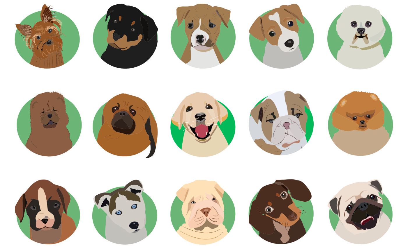
Figure 13.1: Examples of different breeds of the species Canus familiaris. Image is in the Public Domain.
Intraspecific variation can be attributed to pre-defined classifications (breed, age, sex) or to random differences among individuals. Anyone with two pets of the same breed, age, and sex is likely to be able to list off a variety of ways in which their pets differ whether these differences be size, temperament, or dietary preferences. These differences can be driven by genetics (“nature”) and environmental factors (“nurture”).
In the case of Canus familiaris and other domesticated species, intraspecific variation is created and maintained by artificial selection by humans. Artificial selection is not necessary for the development and maintenance of intraspecific variation, however. In natural populations, considerable variation exists between individuals of the same species for both intrinsic and extrinsic reasons, causing differences in the way that conspecifics look, behave, and respond to natural selection pressures, such as predation risk, food availability, and novel environments (Bolnick et al. 2003). This variation plays an important role in the dynamics of populations, communities, and ecosystems.
In addition to individuals varying in their average traits, ecologists are increasingly interested in how individuals vary in the flexibility of these traits. That is, how much and in what way do individuals change their behavior, morphology, physiology, or phenology in response to changing internal or external stimuli? This flexibility in behavior is known as phenotypic plasticity (Figure 13.2).

Figure 13.2: An example of intraspecific variation in a species of finch consuming seeds. Figure 13.2A depicts the overall one-dimensional niche of this species (black dashed line) in terms of the seed sizes that they consume. Within this niche, different individuals (lined of varying colors) specialize on different size seeds, showing intraspecific variation. Figure 13.2B shows how two of these individuals (Individual A and Individual B) vary their resource use with changes in resource availability. Here, Ind B shows greater phenotypic plasticity because this individual alters their resource use to a greater extent when resources change (i.e., the slope of the line for Ind B is greater).
Generally, phenotypic plasticity is more important for immobile organisms (e.g. plants) than mobile organisms (e.g. most animals), as mobile organisms can often move away from unfavorable environments (Schlichting 1968). Nevertheless, mobile organisms also have at least some degree of plasticity in at least some aspects of the phenotype. One mobile organism with substantial phenotypic plasticity is Acyrthosiphon pisum of the aphid family, which exhibits the ability to interchange between asexual and sexual reproduction, as well as growing wings between generations when plants become too populated (Figure 13.3) (Eisen et al. 2010).
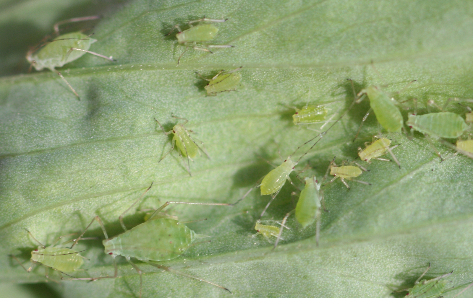
Figure 13.3: Acyrthosiphon pisum by Whitney Cranshaw is Licensed under CC SA 3.0.
The Importance of Understanding Intraspecific Variation in a Changing World
Given that there is substantial variation among individuals, it is inevitable that when presented with anthropogenic stressors, individuals from the same species will respond in different ways (Bolnick et al. 2011). These varied responses may define the difference between success and failure; the likelihood of mortality or the ability to emigrate, to adapt through genetic changes, or to respond via phenotypic plasticity (Engås et al. 1996; Höglund et al. 2008; Cripps et al. 2014).
Intraspecific variation in responses can also have far-reaching impacts on the population dynamics, community structure and ecosystem function of entire groups of animals (Post et al. 2008; Rudman et al. 2015; Charette and Derry 2016; Des Roches et al. 2017). Indeed, in some cases intraspecific variation can have a greater influence than interspecific differences on overall community responses to environmental change (Crutsinger et al. 2006; Siefert and Ritchie 2016; Raffard et al. 2019).
Furthermore, varied responses set the stage for future evolution, as the cohort of individuals capable of reproducing following an anthropogenic stress event defines the evolutionary potential of the population that remains after the disturbance event (Medina et al. 2007; Bijlsma and Loeschcke 2012). To consider only “mean” responses to anthropogenic stressors is therefore to underappreciate the likely consequences of the disturbance; a lack of population-level impacts may be masking more subtle but important within-population changes. Conversely, consideration of intraspecific variation facilitates a more comprehensive understanding of the impacts of anthropogenic stressors on animals, the likely consequences for wider ecosystems, and the best management strategies to address these changes.
While phenotypic plasticity can play a role in the persistence of individuals under changing environmental conditions (Nicotra et al., 2010), the extent of phenotypic plasticity can be limited by ecological and evolutionary constraints (Valladares et al., 2007). The distribution of traits within a community is expected to reflect variation around a mean optimal phenotype for fitness and/or growth rate (Norberg et al., 2001; Enquist et al., 2015). This idea follows from a central paradigm in ecology (Whittaker, 1972) and evolutionary biology (Levins, 1968) where observed shifts in phenotypes, species’ abundances, and composition across environmental gradients reflect the arrangement of phenotypes or species that maximizes fitness in different environments. Abiotic filters such as temperature or moisture that limit successful survival strategies promote convergence of traits around this optimal local phenotype (Keddy, 1992; Weiher and Keddy, 1999; Violle et al., 2012).
On the other hand, when competitive interactions are a dominant factor in species survival or environmental conditions are highly variable at a scale smaller than the study unit, there could be advantages to expressing more variable phenotypes that are not clumped at the optimal phenotype (Pacala and Tilman, 1994; Grime, 2006). However, tests of this theory have shown mixed results with some evidence for higher fitness (Lajoie and Vellend, 2018) or occurrence (Muscarella and Uriarte, 2016) when species are nearer the community trait mean while other cases showed no tendency for species in their preferred habitats to have trait values closer to the community mean (Mitchell et al., 2018). The importance of intraspecific variation in this dynamic is also unclear.
The Study of Intraspecific Variation
Two of the most studied aspects of intraspecific variation are variation in the behavior of individuals within a species, often called “animal personality”, and variation in the diet of individuals within a species, often called “individual specialization”.
Animal Personality
Personality in animals has been investigated across a variety of different scientific fields including agricultural science, animal behavior, anthropology, psychology, veterinary medicine, and zoology (Gosling 2001). Thus, the definition for animal personality may vary according to the context and scope of study. However, there is recent consensus in the literature for a broad definition that describes animal personality as individual differences in behavior that are consistent across time and ecological context (Wolf et al. 2012). Here, consistency refers to the repeatability of behavioral differences between individuals and not a trait that presents itself the same way in varying environments (Réale et al. 2007; Stamps and Groothuis 2010).
Animal personality traits are measurable and are described in over 100 species (Carere and Locurto 2011). Personality in animals has also been referred to as animal disposition, coping style, and temperament (Gosling 2001). There are also personality norms through the species, often found between genders (Gosling 2008). The diversity of animal personality can be compared in cross-species studies, demonstrating its pervasiveness in the evolutionary process of animals (Gosling 2001). Research on animal personality variation has been burgeoning since the mid 1990s (Kralj-Fišer and Schuett 2014). Recent studies have focused on its proximate causation and the ecological and evolutionary significance of personality in animals (Stamps and Groothuis 2010).
Example: The spider Anelosimus studiosus forms groups in which some females show an aggressive personality type and engage more in colony defense and prey capture, while others are docile and engage more in brood care. Groups containing both these two different personalities have better fitness than groups of only one personality type. This is because aggressive females are more efficient at foraging, web construction and defense, while docile females are better at raising the young. When groups contain a mix of both personalities, overall group performance is improved benefiting all group members (Grinsted and Bacon 2014). In the social spider Stegodyphus dumicola individuals differ in their boldness, with bolder individuals having a greater risk appetite. Boldness changes were found to relate to social interactions with nest mates, indicating that individual personality is more plastic in groups (Hunt et al. 2018).
Animal personality vs. human personality
The extent of personality phenomenon considered when examining animal personality is significantly reduced compared to those studied in humans. Concepts such as personal objects, identity, attitudes and life stories are not considered relevant in animals. Similarly, any approach that requires the subject to explain motives, beliefs or feelings is not applicable to the study of animal behavior (Gosling 2001).
The study of animal personality is largely based on the observation and investigation of behavioral traits. In an ecological context, traits or ‘characters’ are attributes of an organism that are shared by members of a species. Traits can be shared by all or only a portion of individuals in a population. For example, studies in animal personality often examine traits such as aggressiveness (antagonistic interactions with other individuals of the same species), boldness (reaction to risky situations), exploration (reaction to new situations), activity (movement in a familiar environment), and sociality (positive interactions with other individuals of the same species).
Quantifying Intraspecific Variation in Behavior: Repeatability
Repeatability refers to the fraction of variation in a population that is owed to differences between individuals. Repeatability estimates are one of the most widely used statistical tools that can quantify consistent individual differences in behavior (Biro et al. 2015). Formally,

where, is variance among individuals and is the variance within individuals over time (Leclerc et al. 2016). In a meta-analysis of published, peer-reviewed repeatability estimates, reviewers found that, in general, approximately 35% of behavioral variation among individuals could be attributed to individual differences (Bell et al. 2009).
 is variance among individuals and
  is the variance within individuals over time (Leclerc et al. 2016). In a meta-analysis of published, peer-reviewed repeatability estimates, reviewers found that, in general, approximately 35% of behavioral variation among individuals could be attributed to individual differences (Bell et al. 2009).
Evolutionary potential
The degree of variation in a population has been determined to influence the direction and outcome of natural selection. Most scientific research has focused on genetic and phenotypic variation or differences in resource use; however, variation in consistent behaviors (i.e. personality) also has important evolutionary consequences. For example, personality in animals can affect the way individuals interact with their environment and with each other which can affect the relative fitness of individuals (Biro and Stamps 2008). Therefore, personality can influence selection. Also, behavioral traits are more dynamic which may allow an animal to adapt more quickly which, in turn, can speed up the rate of evolution (Wolf and Weissing 2012).
Further, natural or artificial selection cannot act on personality unless there is a mechanism for its inheritance. In rhesus macaques (Maccaca mulatta), the personality traits of Meek, Bold, Aggressive, Passive, Loner and Nervous have heritability values of 0.14 to 0.35, thus indicated that there is some genetic basis to the expression of personality traits in animals. In apes, including humans, heritability estimates of personality dimensions range from 0.07 to 0.63 (Brent et al. 2014). In horses, heritability estimates range mostly between h2=0.15 and h2=0.40 for traits assessed in personality tests. Values at this level are considered as "promising" for artificial selection (Brent et al. 2014).
Reaction norms help us study personality and plasticity
A potentially useful way to understand how individual variation interacts with the factors known to influence phenotypic traits is to view a phenotypically plastic trait using a reaction norm. A reaction norm is the set of phenotypes a genotype/individual could express across a set of environments (Via et al. 1995). The reaction norm has a long history for studying phenotypic variation (Stearns 1989; Pigliucci 2001). Using a reaction norm model (see below) we can study individual variation in a phenotypic trait in terms of individual deviation from the population mean, as well as individual variation from the mean population response to the environmental (individual phenotypic plasticity). A reaction norm approach can also allow insight into how and why individuals vary in different dimensions, both in their mean expression of a trait (reaction norm height) and the plasticity of the trait (reaction norm slope). The basic reaction norm to study how a trait (y) varies with some environmental factor (E) can be written as:
yij = μ + βEj + pi + pEiEj + εij
where yij is the phenotype of individual i on occasion j. This equation contains two main effects, the fixed effects and the random effects, and the residual error effects. The fixed effects represent the population average response of the trait (y) to the change in the environment (E). The fixed effects include the variables μ, which is the population mean phenotype in the average environment, and β, which is the population mean slope of y on E. The random effects represent individual phenotypic differences from the population average height and slope. The random effects include the variables pi, which is the permanent deviation of individual i from the mean population phenotype independent of E (personality: individual reaction norm height), and pEi, which is the deviation of individual i from the population average slope (individual plasticity). The best way to interpret this equation may be to visualize what each component means in graphical form (Figure 13.4). The reaction norm approach allows us to estimate the variance in a trait that is due to the effect of individual variation. We can also test for significant differences in the variance in height of the individual reaction norms (Vp) to see if individuals differ in their average phenotype, as well as test for differences in the variance of individual slopes of the reaction norms (VpE; Figure 13.5).
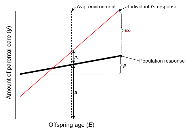
Figure 13.4: This diagram represents the basic reaction norm model, where the phenotype y is the amount of parental care and the environment E is the age of offspring. The variable μ represents the population mean phenotype in the average environment, and β is the population mean slope. The random effects are represented by pi, which is the permanent deviation of individual i from the mean population phenotype (personality: individual reaction norm height), and pEi, which is the deviation of individual i from the population average slope (individual plasticity).
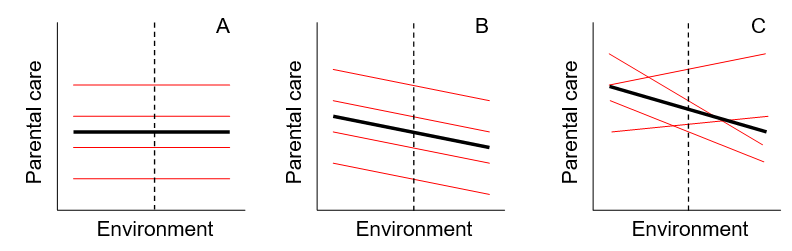
Figure 13.5: These diagrams represent examples of reaction norms with different degrees of variation. The thick black line is the mean population response to the environment, and each thin red line represents an individual’s phenotype across the environment. The diagrams show that: (A) there is individual variation in the phenotype (personality: heights of the red lines), but that there is no phenotypic plasticity, (B) there is individual variation in the phenotype (personality: heights of the red lines), there is population-level phenotypic plasticity (slopes of the red lines are non-zero), but individuals do not differ in their response to the environment (slopes of the red lines are equal), and (C) there is individual variation in the phenotype (personality: heights of the red lines), there is population-level phenotypic plasticity (slopes of the red lines are non-zero), and individuals differ in their response to the environment (individual plasticity: slopes of the red lines vary).
Individual Specialization in Foraging and Diet
Individuals can vary in the quantity of resources they consume, the type of resources they consume, and how they obtain these resources (i.e., in their foraging behavior). This variation in diet and foraging behavior can be linked to animal personality. For example, more aggressive individuals are likely to benefit from social dominance that allows them access to higher quality resources than subordinate individuals (Toscano et al. 2016).
Individual specialization is specifically used to describe variation in diet among individuals that is not driven by a priori factors like morphology, sex, or age. In the formula below, diet is driven by variation due to sex, age, morphology, and random differences among individuals; these random differences represent intraspecific variation in diet (Bolnick et al. 2003).
diet = sex + age + morphology + random differences
Measuring Intraspecific Variation
Intraspecific variation in diet and foraging is studied using traditional tools (e.g., observation, gut content analysis) as well as more modern tools such as stable isotope analysis and animal tagging. These tools have considerable advantages in studying animal foraging behavior (tagging) and diet (stable isotope analysis).
Tagging data is particularly useful because it provides high-frequency, continuous data that allows researchers to determine multiple ways in which animals vary in their foraging (e.g., foraging distance, foraging location, diving depth) and how they alter this behavior when conditions change. In Figure 13.6, for example, individual great black-backed gulls (Larus marinus) vary in where they forage and in how they shift their foraging locations when food availability declines.

Figure 13.6: Differences in space use of individual great black-backed gulls (Larus marinus) foraging on capelin (Mallotus villosus), a small schooling fish species, in Newfoundland, Canada. Individuals vary not only in the average size and location of their foraging areas, but also in how much they shift these areas from high food availability (High capelin; purple) to low food availability (Low capeline; orange). Murre (Uria aalge) are another species of seabird that breed in this region and consume capelin.
The concept of intraspecific variation in diet is closely related to the concept of generalist versus specialist populations. In a specialist population, all individuals use similar resources and a narrow range of resources. Generalist populations use a wide range of resources, but this can be due to 1) individuals in the population all using a wide range of resources (true generalists) or 2) individuals in the population specializing on different resources, so that the overall population niche is wide but individual niches are not (generalist-specialists). In Figure 13.2, for example, the generalist population is made up of specialists. More information on these concepts can be found in the chapter on animal behavior, and specifically in the sections on Animal Foraging and Animal Movement.
Individual variation in diet is often studied using stable isotope analysis. Stable isotope analysis of diet is based on the idea that “you are what you eat”. In other words, your elemental composition is determined by that of what you consume. All biologically active elements exist in a number of different isotopic forms, of which two or more are stable. For example, most carbon is present as 12C, with approximately 1% being 13C. The ratio of the two isotopes may be altered by biological and geophysical processes, and these differences can be used in a number of ways by ecologists. The main elements used in diet studies are carbon and nitrogen (Michener and Lajtha 2007).
Carbon-13
Carbon isotopes aid us in determining the primary production source responsible for the energy flow in an ecosystem. The transfer of 13C through trophic levels remains relatively the same, except for a small increase (an enrichment < 1 ‰). Large differences of δ13C between animals indicate that they have different food sources or that their food webs are based on different primary producers (i.e. different species of phytoplankton, marsh grasses.) Because δ13C indicates the original source of primary producers, the isotopes can also help us determine shifts in diets, both short term, long term or permanent. These shifts may even correlate to seasonal changes, reflecting phytoplankton abundance (Michener and Kaufman 2007). Scientists have found that there can be wide ranges of δ13C values in phytoplankton populations over a geographic region. While it is not quite certain as to why this may be, there are several hypotheses for this occurrence. These include isotopes within dissolved inorganic carbon pools (DIC) may vary with temperature and location and that growth rates of phytoplankton may affect their uptake of the isotopes.
Nitrogen-15
Nitrogen isotopes indicate the trophic level position of organisms (reflective of the time the tissue samples were taken). There is a larger enrichment component with δ15N because its retention is higher than that of 14N. This can be seen by analyzing the waste of organisms (Michener and Kaufman 2007). Cattle urine has shown that there is a depletion of 15N relative to the diet (Kelly et al. 2002). As organisms eat each other, the 15N isotopes are transferred to the predators. Thus, organisms higher in the trophic pyramid have accumulated higher levels of 15N ( and higher δ15N values) relative to their prey and others before them in the food web. Numerous studies on marine ecosystems have shown that on average there is a 3.2‰ enrichment of 15N vs. diet between different trophic level species in ecosystems (Michener and Kaufman 2007). In the Baltic sea, Hansson et al. (1997) found that when analyzing a variety of creatures (such as particulate organic matter (phytoplankton), zooplankton, mysids, sprat, smelt and herring,) there was an apparent fractionation of 2.4‰ between consumers and their apparent prey (Doucett et al. 2007).
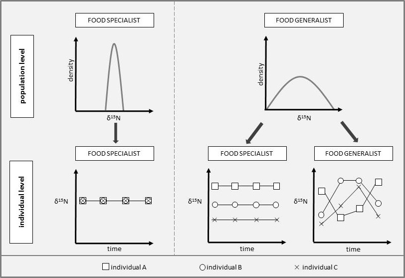
In addition to comparing signatures across individuals, stable isotopes can be used to examine phenotypic plasticity because different tissue types (fur, blood, muscle) have different turnover rates and therefore reflect the diet of individuals across different timescales (Figure 13.7). Therefore, if multiple tissue types are collected from an individual, the diet of that individual can be examined over multiple temporal scales to determine how much variation there is within the individual’s diet (i.e., how flexible their diet is).
Figure 13.7: Conceptual diagram of how individuals can contribute to the population's dietary niche. Specialized populations consist of specialized individuals which all consume certain resources (left). Therefore, their total dietary niche represents a small dietary variation within and between individuals. In contrast, generalistic populations can consist either of specialized or generalistic individuals (right). In this case, specialized individuals show small dietary variation within individuals, but a large dietary variation between individuals leads to a broad overall resource spectrum and dietary variation at the population level. If individuals of a generalistic population forage generalistic then those are characterized by a large within-individual dietary variation. Taken from Scholz et al. 2020.
Quantifying Intraspecific Variation
Whether using isotope data or another continuous indicator of resources use (e.g., seed size; Figures 13.2 and 13.8), intraspecific variation can be quantified by comparing the average width of the individual niche (WIC - within individual component of niche variation) to the total niche width (TNW). The total niche width is equal to the WIC plus the BIC, or the between-individual component of niche variation (Bolnick et al. 2003). When BIC/TNW is relatively high, there is high intraspecific variation (i.e., individuals have consistent dietary preferences but these preferences vary across individuals) and the population is a specialist-generalist population (Figure 13.8A). When WIC/TNW is relatively high, all individuals show considerable variation in diet but have highly overlapping niches and the population is a true population of generalists (Figure 13.8B).
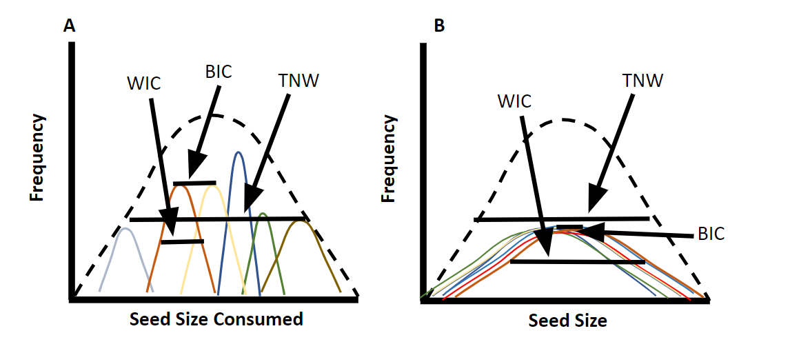
Figure 13.8: An example of intraspecific variation in a species of finch consuming seeds. Figure 13.8A shows a generalist population of specialists. While the range of seed sizes consumed by the population is large, individuals within the population each only consume a small range of seed sizes. Therefore, the within-individual component of variation (WIC) is a small proportion of the total niche width (TNW) and intraspecific variation is high. Figure 13.8B shows a generalist population of generalists. Since all individuals within this population consume a wide range of seed sizes, the WIC is high and intraspecific variation is low.
Intraspecific Variation in the Diet of Red Foxes
Some carnivores are known to survive well in urban habitats, yet the underlying behavioral tactics are poorly understood. One likely explanation for the success in urban habitats might be that carnivores are generalist consumers. However, urban populations of carnivores could as well consist of specialist feeders.
Scholz et al. (2020) compared the isotopic specialization of red foxes in urban and rural environments, using both a population and an individual level perspective. They measured stable isotope ratios in increments of red fox whiskers and potential food sources. Their results reveal that red foxes have a broad isotopic dietary niche and a large variation in resource use (Figure 13.9).
Despite this large variation, they found significant differences between the variance of the urban and rural population for δ13C as well as δ15N values, suggesting a habitat-specific foraging behavior. Although urban regions have more heterogeneous land cover than rural regions, the dietary range of urban foxes was smaller compared with that of rural conspecifics. Moreover, the higher δ13C values and lower δ15N values of urban foxes suggest a relatively high input of anthropogenic food sources.
The diet of most individuals remained largely constant over a longer period. The low intraindividual variability of urban and rural red foxes suggests a relatively constant proportion of food items consumed by individuals. Urban and rural foxes utilized a small proportion of the potentially available isotopic dietary niche as indicated by the low within-individual variation compared to the between-individual variation. Scholz et al. (2020) conclude that generalist fox populations consist of individual food specialists in urban and rural populations.
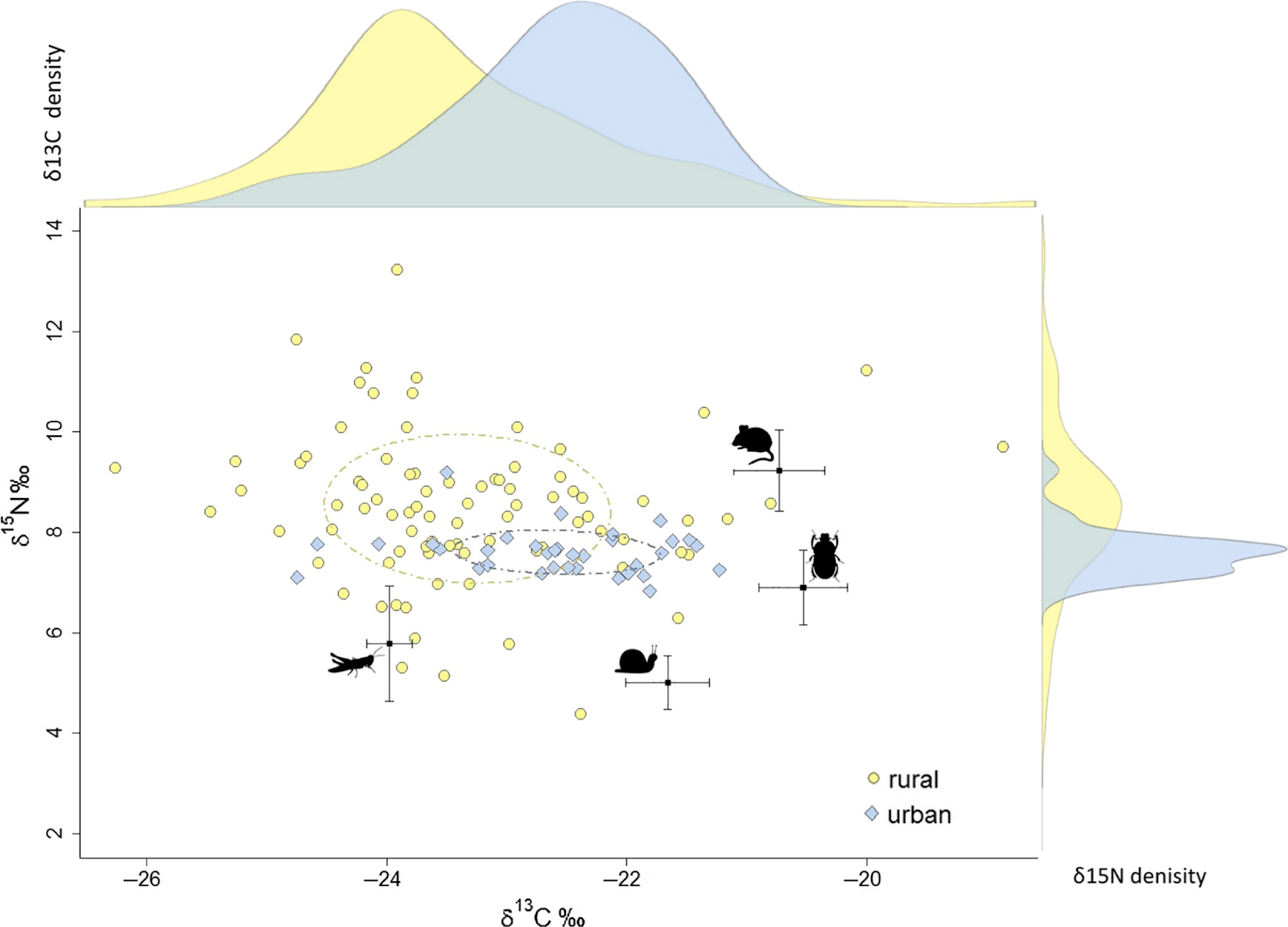
Figure 13.9: Isospace and density plot for raw δ13C and δ15N values of urban (blue diamonds) and rural (yellow circles) red foxes whisker samples (n = 119) from Berlin and Brandenburg, Germany. Dashed ellipses represent SEAc of the urban (blue) and rural (yellow) fox population. Black dots show trophic corrected mean (±SE bars) δ13C and δ15N values for the four prey taxa including (1) grasshopper, (2) land slug, land snail, earthworm (pooled together), (3) dor beetle, and (4) house mouse. Taken from Scholz et al. 2020.
While ecological studies sometimes focus on variation among species (interspecific variation) there is often substantial variation in the traits and behaviors of individuals within a species (intraspecific variation). Individuals might vary in their mean phenotype and in how much their phenotype responds to changes in their environment (phenotypic plasticity). Two key fields of research into intraspecific variation include animal personality, variation in the behavior of individuals within a species, and individual specialization, variation in the diet of individuals within a species.
Attributions
This chapter was written by N. Gownaris and D. Wetzel with text taken from the following CC-BY resources:
- Isotope analysis by Wikipedia, the free encyclopedia
- Phenotypic plasticity by Wikipedia, the free encyclopedia
- Personality in Animal by Wikipedia, the free encyclopedia
- Harding, H. R., Gordon, T. A., Eastcott, E., Simpson, S. D., & Radford, A. N. (2019). Causes and consequences of intraspecific variation in animal responses to anthropogenic noise. Behavioral Ecology, 30(6), 1501-1511. https://doi.org/10.1093/beheco/arz114
- Henn, J. J., Buzzard, V., Enquist, B. J., Halbritter, A. H., Klanderud, K., Maitner, B. S., ... & Vandvik, V. (2018). Intraspecific trait variation and phenotypic plasticity mediate alpine plant species response to climate change. Frontiers in Plant Science, 9, 1548. https://doi.org/10.3389/fpls.2018.01548
- Scholz, C., Firozpoor, J., Kramer‐Schadt, S., Gras, P., Schulze, C., Kimmig, S. E., ... & Ortmann, S. (2020). Individual dietary specialization in a generalist predator: A stable isotope analysis of urban and rural red foxes. Ecology and Evolution, 10(16), 8855-8870. https://doi.org/10.1002/ece3.6584
References
Bell, Alison M.; Hankison, Shala J.; Laskowski, Kate L. (2009). "The repeatability of behaviour: a meta-analysis". Animal Behaviour. 77 (4): 771–783. doi:10.1016/j.anbehav.2008.12.022. PMC 3972767. PMID 24707058.
Bijlsma R, Loeschcke V. 2012. Genetic erosion impedes adaptive responses to stressful environments. Evol Appl. 5:117–129.
Biro, Peter A.; Stamps, Judy A. (2008). "Are animal personality traits linked to life-history productivity?". Trends in Ecology & Evolution. 23 (7): 361–368. doi:10.1016/j.tree.2008.04.003. PMID 18501468.
Biro, Peter A.; Stamps, Judy A. (2015). "Using repeatability to study physiological and behavioural traits: ignore time-related change at your peril". Animal Behaviour. 105: 223–230. doi:10.1016/j.anbehav.2015.04.008. S2CID 53203738.
Bolnick DI, Amarasekare P, Araújo MS, Bürger R, Levine JM, Novak M, Rudolf VHW, Schreiber SJ, Urban MC, Vasseur D. 2011. Why intraspecific trait variation matters in community ecology. Trends Ecol Evol. 26:183–192.
Bolnick, D. I., Svanbäck, R., Fordyce, J. A., Yang, L. H., Davis, J. M., Hulsey, C. D., & Forister, M. L. (2003). The ecology of individuals: incidence and implications of individual specialization. The American Naturalist, 161(1), 1-28.
Carere, C. & Locurto, C. (2011). "Interaction between animal personality and animal cognition". Current Zoology. 57 (4): 491–498. doi:10.1093/czoolo/57.4.491.
Charette C, Derry AM. 2016. Climate alters intraspecific variation in copepod effect traits through pond food webs. Ecology. 97:1239–1250.
Cripps G, Lindeque P, Flynn KJ. 2014. Have we been underestimating the effects of ocean acidification in zooplankton? Glob Chang Biol. 20:3377–3385.
Crutsinger GM, Collins MD, Fordyce JA, Gompert Z, Nice CC, Sanders NJ. 2006. Plant genotypic diversity predicts community structure and governs an ecosystem process. Science. 313:966–968.
Des Roches S, Post DM, Turley NE, Bailey JK, Hendry AP, Kinnison MT, Schweitzer JA, Palkovacs EP. 2017. The ecological importance of intraspecific variation. Nat Ecol Evol. 2:57–64.
Doucett, Richard R.; Marks, Jane C.; Blinn, Dean W.; Caron, Melanie; Hungate, Bruce A. (June 2007). "Measuring Terrestrial Subsidies to Aquatic Food Webs Using Stable Isotopes of Hydrogen". Ecology. 88 (6): 1587–1592. doi:10.1890/06-1184. PMID 17601150.
Engås A, Løkkeborg S, Ona E, Soldal AV. 1996. Effects of seismic shooting on local abundance and catch rates of cod (Gadus morhua) and haddock (Melanogrammus aeglefinus). Can J Fish Aquat Sci. 53:2238–2249.
Enquist, B. J., Norberg, J., Bonser, S. P., Violle, C., Webb, C. T., Henderson, A., et al. (2015). Scaling from traits to ecosystems: developing a general trait driver theory via integrating trait-based and metabolic scaling theories. Adv. Ecol. Res. 52, 249–318. doi: 10.1016/bs.aecr.2015.02.001
Gosling, S. D. (January 2001). "From mice to men: what can we learn about personality from animal research?". Psychological Bulletin. 127 (1): 45–86. doi:10.1037/0033-2909.127.1.45. ISSN 0033-2909. PMID 11271756.
Gosling, Samuel (2008). "Personality in Non-human Animals" (PDF). Social and Personality Psychology Compass. 2 (2): 985–1001. doi:10.1111/J.1751-9004.2008.00087.X. S2CID 43114990. Archived from the original (PDF) on 19 November 2018. Retrieved 18 November 2018.
Grime, J. P. (2006). Trait convergence and trait divergence in herbaceous plant communities?: mechanisms and consequences stable: trait convergence and trait divergence in her. J. Veg. Sci. 17, 255–260. doi: 10.1111/j.1654-1103.2006.tb02444.x1
Grinsted, L. & Bacon, J.P. (2014). "Animal behaviour: Task differentiation by personality in spider groups". Current Biology. 24 (16): R749–R751. doi:10.1016/j.cub.2014.07.008. PMID 25137587.
Höglund E, Gjøen H-M, Pottinger TG, Øverli Ø. 2008. Parental stress-coping styles affect the behaviour of rainbow trout Oncorhynchus mykiss at early developmental stages. J Fish Biol. 73:1764–1769.
Hunt, ER.; et al. (2018). "Social interactions shape individual and collective personality in social spiders". Proceedings of the Royal Society B. 285 (1886): 20181366. doi:10.1098/rspb.2018.1366. PMC 6158534. PMID 30185649.
International Aphid Genomics Consortium (February 2010). Eisen JA (ed.). "Genome sequence of the pea aphid Acyrthosiphon pisum". PLOS Biology. 8 (2): e1000313. doi:10.1371/journal.pbio.1000313. PMC 2826372. PMID 20186266
Keddy, P. A. (1992). Assembly and response rules: two goals for predictive community ecology. J. Veg. Sci. 3, 157–164. doi: 10.2307/3235676
Kelly, Jeffrey F.; Atudorei, Viorel; Sharp, Zachary D.; Finch, Deborah M. (1 January 2002). "Insights into Wilson's Warbler migration from analyses of hydrogen stable-isotope ratios". Oecologia. 130 (2): 216–221. Bibcode:2002Oecol.130..216K. doi:10.1007/s004420100789. PMID 28547144. S2CID 23355570.
Kralj-Fišer, S. & Schuett, W. (2014). "Studying personality variation in invertebrates: Why bother?". Animal Behaviour. 91: 41–52. doi:10.1016/j.anbehav.2014.02.016. S2CID 53171945.
Lajoie, G., and Vellend, M. (2018). Characterizing the contribution of plasticity and genetic differentiation to community-level trait responses to environmental change. Ecol. Evol. 8, 3895–3907. doi: 10.1002/ece3.3947
Leclerc, Martin; Wal, Eric Vander; Zedrosser, Andreas; Swenson, Jon E.; Kindberg, Jonas; Pelletier, Fanie (2016-03-01). "Quantifying consistent individual differences in habitat selection". Oecologia. 180 (3): 697–705. Bibcode:2016Oecol.180..697L. doi:10.1007/s00442-015-3500-6. ISSN 0029-8549. PMID 26597548.
Levins, R. (1968). Evolution in Changing Environments: Some Theoretical Explorations. Princeton, NJ: Princeton University Press.
Medina MH, Correa JA, Barata C. 2007. Micro-evolution due to pollution: possible consequences for ecosystem responses to toxic stress. Chemosphere. 67:2105–2114.
Michener, Robert H; Kaufman, Les (2007). "Stable Isotope Ratios as Tracers in Marine Food Webs: An Update". Stable Isotopes in Ecology and Environmental Science. pp. 238–82. doi:10.1002/9780470691854.ch9. ISBN 978-0-470-69185-4.
Michener, Robert; Lajtha, Kate, eds. (2007-10-08). Stable isotopes in ecology and environmental science (2nd ed.). Blackwell Pub. pp. 4–5. ISBN 978-1-4051-2680-9.
Mitchell, R. M., Wright, J. P., and Ames, G. M. (2018). Species’ traits do not converge on optimum values in preferred habitats. Oecologia 186, 719–729. doi: 10.1007/s00442-017-4041-y
Muscarella, R., and Uriarte, M. (2016). Do community-weighted mean functional traits reflect optimal strategies? Proc. Biol. Sci. 283:20152434. doi: 10.1098/rspb.2015.2434
Nicotra, A. B., Atkin, O. K., Bonser, S. P., Davidson, A. M., Finnegan, E. J., Mathesius, U., et al. (2010). Plant phenotypic plasticity in a changing climate. Trends Plant Sci. 15, 684–692. doi: 10.1016/j.tplants.2010.09.008
Norberg, J. J., Swaney, D. P., Dushoff, J. J., Lin, J. J., Casagrandi, R. R., and Levin, S. A. (2001). Phenotypic diversity and ecosystem functioning in changing environments: a theoretical framework. Proc. Natl. Acad. Sci. U.S.A. 98, 11376–11381. doi: 10.1073/pnas.171315998
Pacala, S., and Tilman, D. (1994). Limiting similarity in mechanistic and spatial models of plant competition in heterogeneous environments. Am. Nat. 143, 222–257. doi: 10.1086/285602
Pigliucci, M. (2001). Phenotypic plasticity: beyond nature and nurture. JHU Press.
Post DM, Palkovacs EP, Schielke EG, Dodson SI. 2008. Intraspecific variation in a predator affects community structure and cascading trophic interactions. Ecology. 89:2019–2032.
Raffard A, Santoul F, Cucherousset J, Blanchet S. 2019. The community and ecosystem consequences of intraspecific diversity: a meta-analysis. Biol Rev. 94:648–661.
Réale, Denis; Reader, Simon M.; Sol, Daniel; McDougall, Peter T.; Dingemanse, Niels J. (2007-05-01). "Integrating animal temperament within ecology and evolution". Biological Reviews. 82 (2): 291–318. doi:10.1111/j.1469-185x.2007.00010.x. hdl:1874/25732. ISSN 1469-185X. PMID 17437562. S2CID 44753594.
Rudman SM, Rodriguez-Cabal MA, Stier A, Sato T, Heavyside J, El-Sabaawi RW, Crutsinger GM. 2015. Adaptive genetic variation mediates bottom-up and top-down control in an aquatic ecosystem. Proc Biol Sci. 282:20151234.
Schlichting CD (1986). "The Evolution of Phenotypic Plasticity in Plants". Annual Review of Ecology and Systematics. 17: 667–93. doi:10.1146/annurev.es.17.110186.003315.
Siefert A, Ritchie ME. 2016. Intraspecific trait variation drives functional responses of old-field plant communities to nutrient enrichment. Oecologia. 181:245–255.
Stamps, J. & Groothuis, T.G. (2010). "The development of animal personality: relevance, concepts and perspectives". Biological Reviews. 85 (2): 301–325. doi:10.1111/j.1469-185x.2009.00103.x. hdl:11370/67a37755-a0d2-41f9-adf7-aec21a63dca5. PMID 19961473. S2CID 33798211.
Stearns, S. C. (1989). The evolutionary significance of phenotypic plasticity. Bioscience, 39(7), 436-445.
Toscano, B. J., Gownaris, N. J., Heerhartz, S. M., & Monaco, C. J. (2016). Personality, foraging behavior and specialization: integrating behavioral and food web ecology at the individual level. Oecologia, 182(1), 55-69.
Valladares, F., Gianoli, E., and Gómez, J. M. (2007). Ecological limits to plant phenotypic plasticity. New Phytol. 176, 749–763. doi: 10.1111/j.1469-8137.2007.02275.x
Via, S., Gomulkiewicz, R., De Jong, G., Scheiner, S. M., Schlichting, C. D., & Van Tienderen, P. H. (1995). Adaptive phenotypic plasticity: consensus and controversy. Trends in ecology & evolution, 10(5), 212-217.
Violle, C., Enquist, B. J., McGill, B. J., Jiang, L., Albert, C. H., Hulshof, C., et al. (2012). The return of the variance: intraspecific variability in community ecology. Trends Ecol. Evol. 27, 244–252. doi: 10.1016/j.tree.2011.11.014
Weiher, E., and Keddy, P. (1999). “Assembly rules as general constraits on community composition,” in Ecological Assembly Rules: Perspecitves, Advances, Retreats, eds E. Weiher and P. A. Keddy (Cambridge: Cambridge University Press), 251–271. doi: 10.1017/CBO9780511542237.010
Whittaker, R. (1972). Evolution and measurement of species diversity. Taxon 21, 213–251. doi: 10.2307/1218190
Wolf, Max; Weissing, Franz J. (2012). "Animal personalities: consequences for ecology and evolution". Trends in Ecology & Evolution. 27 (8): 452–461. doi:10.1016/j.tree.2012.05.001. PMID 22727728.