14.2: Basic Principles of Metabolic Control Analysis (MCA)

Search Fundamentals of Biochemistry

Learning Goals (ChatGPT o3-mini)

1. Conceptualize Metabolic Control Analysis (MCA):

   • Define MCA and explain why enzyme kinetics in complex metabolic pathways require a systems-level approach.
   • Describe the challenges posed by the multiple steps, rate constants, and chemical species involved in enzyme-catalyzed reactions.

2. Differentiate Between Equilibrium and Steady-State Conditions:

   • Contrast equilibrium conditions (where no net change in reactant or product concentrations occurs) with steady state in open systems (where input equals output).
   • Explain the significance of steady state in cellular metabolism and why it is more relevant to in vivo conditions than equilibrium.

3. Apply Differential Equations to Model Metabolic Reactions:

   • Write ordinary differential equations (ODEs) for simple and complex reaction schemes, including unimolecular and bimolecular reactions.
   • Interpret the ODEs used to describe the time-dependent concentration changes of reactants, intermediates, and products in metabolic pathways.

4. Understand and Analyze Enzyme Kinetics Using Simulation Tools:

   • Utilize computational programs such as VCell and COPASI to simulate progress curves (concentration vs. time) for enzyme-catalyzed reactions.
   • Compare simulation results for isolated enzyme reactions with those embedded in metabolic “mini-pathways” and evaluate how pathway context alters apparent equilibrium constants.

5. Relate In Vitro vs. In Vivo Kinetics:

   • Explain how experimental approaches (varying substrate or inhibitor concentrations in vitro) differ from the dynamic conditions encountered in vivo, where flux and steady-state concentrations govern enzyme behavior.
   • Discuss how the concept of flux (J) provides a more accurate description of pathway kinetics in a cellular context.

6. Interpret the Mathematical Derivation of Net Reaction Rates:

   • Follow the derivation of the reversible Michaelis–Menten equation under rapid equilibrium conditions and understand the roles of dissociation constants (K_S and K_P).
   • Explain why the net forward rate of a reversible reaction cannot be determined by a simple subtraction of forward and reverse rates.

7. Analyze the Impact of Inhibitors on Enzyme Kinetics:

   • Distinguish between simple enzyme kinetics and competitive inhibition models by comparing their derived equations.
   • Apply knowledge of inhibition parameters (K_I) to understand how inhibitors alter the net rate of enzymatic reactions.

8. Examine the Role of Computational Models in Systems Biology:

   • Discuss how complex pathways, such as yeast glycolysis, are modeled computationally using curated databases (e.g., Biomodels) and the integration of experimental data.
   • Evaluate how branching reactions and additional pathway components improve the accuracy of simulations relative to experimental in vivo fluxes.

9. Develop Practical Skills in Parameter Variation and Sensitivity Analysis:

   • Practice modifying kinetic parameters (e.g., rate constants, substrate concentrations) in simulation programs to observe their effects on the time-course graphs of metabolite concentrations.
   • Interpret how changes in model parameters influence the steady-state and overall flux of the pathway.

10. Integrate Theoretical and Practical Aspects of Metabolic Control:

    • Synthesize the mathematical derivations, computational simulations, and experimental differences to build a comprehensive understanding of how metabolic pathways are regulated at the systems level.
    • Critically assess the limitations of in vitro enzyme kinetics when applied to the dynamic conditions of living cells.

These learning goals aim to guide students through the theoretical underpinnings and practical applications of metabolic control analysis, equipping them with the skills necessary to bridge the gap between individual enzyme behavior and the integrated function of metabolic networks.

Introduction to Metabolic Control Analysis

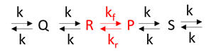
Enzyme kinetics is difficult, in part due to the complicated mathematical derivations, the number of chemical species involved (an enzyme and all its substrates and products), the number of steps in the mechanism, and numerous rate, kinetic, and dissociation constants. An example of such a “complicated” reaction explored earlier is shown in Figure \(\PageIndex{1}\).

 

Figure \(\PageIndex{1}\): Chemical Equations for an enzyme-catalyzed reaction with a covalent E-intermediate

\begin{equation}
v=\frac{\frac{k_2 k_3}{k_2+k_3}\left(E_0\right)(S)}{\left[\frac{k_3}{k_2+k_3}\right] K_S+S}=\frac{k_{c a t}\left(E_0\right)(S)}{K_M+S}
\end{equation}

But single enzymes rarely act in isolation. They are components of complex pathways with many steps, many of which are regulated. To fully understand a reaction, it is important to study the concentrations of all species in the entire pathway as a function of time. Imagine deriving the equations and determining all the relevant concentrations and constants of a pathway such as glycolysis!

To study enzyme kinetics in the lab, you have to spend much time developing assays to measure how the concentration of species changes as a function of time, to be able to measure the initial velocities of an enzyme-catalyzed reaction. However, in networks of interconnected metabolic reactions, the concentration of certain species in the system may remain constant. How can this happen? Two simple examples might help explain how.

Example 1: There is no change in input or output from a given reaction. This would occur in a closed system for a reversible reaction at equilibrium.

For a reversible reaction of reactant R going to product P (R ↔ P) with forward and reverse first-order rate constants, the following equation can be written at equilibrium:

\begin{equation}
\begin{gathered}
v_f=k_1 R=k_2 P \\
K_{e q}=\frac{P_{e q}}{R_{e q}}=\frac{k_1}{k_2}
\end{gathered}
\end{equation}

At equilibrium, \(R\) and \(P\) don’t change.

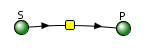
Example 2: Consider the reaction as part of a pathway of reactions (like an open system). Now, imagine a nonzero input to form reactant R and a nonzero output that consumes product P, as shown in Figure \(\PageIndex{2}\).

Figure \(\PageIndex{2}\): Reactant R conversion to Product P with preceding and following steps

If the input and output rates are the same, the concentrations of R and P would remain constant over time. This would lead to a steady state but not equilibrium species concentrations.

The Steady State - A Threshold Biochemistry Concept

Students often struggle to understand the concept of steady state and recognize when it may prevail under specific conditions.

in vitro vs. in vivo

In his book Fundamentals of Enzyme Kinetics, Cornish-Bowden discusses the key differences between enzyme kinetics performed in test tubes (in vitro) and what occurs in cells (in vivo). We've discussed this previously, but it's essential to revisit it now. The conditions under which the enzymes are studied (in vitro) and operate (in vivo) are very different.

• In vitro (in the lab), the enzyme is held at a constant concentration while the substrate is varied (i.e, the substrate concentration is the independent variable). The substrate concentration determines the velocity. When inhibition is studied, the substrate varies while the inhibitor is held constant at several different fixed concentrations.
• In vivo (within the cell), the velocity may be maintained at a relatively constant level in a pathway.  This means that the velocity determines the substrate concentration! You may have to repeat this sentence many times in your mind to realize its significance, as it seems to contradict all the kinetics you studied in many courses!  To avoid a bottleneck in flux, the substrate can't build up at the enzyme; therefore, the enzyme processes it in a steady-state fashion to produce the product, as determined by the Michael-Menten equation.

These differences are vastly underappreciated and not widely understood by students and instructors alike.

Additionally, we confound our efforts in helping students understand the steady state by focusing almost exclusively on presenting initial rate v₀ vs [S] curves when the substrate concentration is changed. Then, instructors expect students to magically understand the steady state when substrate levels in pathways don’t change. It’s a big leap out of this box. We can help students better understand the steady state by shifting to progress curves (concentrations vs time), which are easily constructed using programs such as VCell and Copasi.

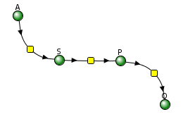
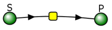
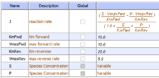
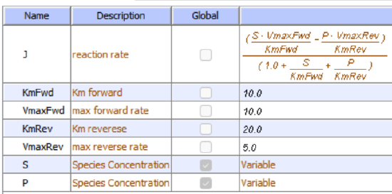
Let's use Vcell to analyze a very simple reversible enzyme in isolation, S ↔ P. Then we will place that same enzyme into a "mini" pathway, A ↔ S ↔ P ↔ Q, in which there is one preceding reactant, A, and one following product, Q, that help control S and P levels. We must start the simulation at a specified concentration, so the default for the simulations is set such that [S] and [A] at time t = 0, S₀ and A₀, are both 5, and the rest are set to 0. Hence, as the simulation begins, concentrations will be adjusted until equilibrium or steady-state concentrations are reached. Table \(\PageIndex{1}\) shows the reaction diagrams and their parameters. Here is the equation for both.

\begin{equation}
\frac{\left(\frac{S \cdot V m a x F w d}{K m F w d}-\frac{P \cdot V m a x R e v}{K m R e v}\right)}{\left(1.0+\frac{S}{K m F w d}+\frac{P}{K m R e v}\right)}
\end{equation}

A reversible enzyme in isolation, S ↔ P	A reversible enzyme for S ↔ P in a mini-pathway A ↔ S ↔ P ↔ Q
Parameter Description Value J Reaction rate S↔P Eq3 KmFwd Km forward 10.0 VmaxFwd Max forward rate 10.0 KmRev Km reverse 20.0 VmaxRev Max reverse rate 5.0 Size Size 50000.0 InitConc Initial concentration for S 5.0	Parameter Description Value J for S↔P Reaction rate S ↔ P, Eq 3 above KmFwd Km forward 10.0 VmaxFwd Max forward rate 10.0 KmRev Km reverse 20.0 VmaxRev Max reverse rate 5.0 J for P↔Q Reaction rate (Kf·P – Kr·Q) Kf Forward rate constant 20.0 Kr Reverse rate constant 2.0 J for A↔S Reaction rate (Kf·A – Kr·S) Kf Forward rate constant 2.0 Kr Reverse rate constant 2.0 Size Size 50000.0 initConc Initial concentration for S 5.0 initConc Initial concentration for P 0.0 initConc Initial concentration for Q 0.0 initConc Initial concentration for A 5.0

Figure \(\PageIndex{3}\): Reaction schemes and parameters for a simple enzyme-catalyzed reversible reaction (left) and the same reaction embedded in a "mini" pathway (right).

Vcell simulation for the isolated enzyme

Remember that an enzyme doesn't change the thermodynamics of a given reaction and hence doesn't alter K_eq. It just speeds up both the forward and the reverse reactions. Hence, you can calculate the K_eq for the reaction condition from the Vcell model time course graph:

\begin{equation}
\mathrm{K}_{\mathrm{eq}}=\frac{[\mathrm{P}]_{\mathrm{eq}}}{[\mathrm{S}]_{\mathrm{eq}}}=\frac{4}{1}=1
\end{equation}

Now you observe that in this reaction, S does change from its initial value, S₀ = 5 (since P₀ = 0). Soon, however, the reaction reaches a dynamic equilibrium, in which both S and P don't change over time.

You could choose a different initial concentration of S and P, rerun the simulation, and calculate K_EQ for the new conditions using the CSV-downloaded spreadsheet data from each run you make. They should be the same.

---

MODEL

Reversible reaction E + S ↔ ES  ↔  EP  ↔  E + P  

Initial values 

Select Load [model name] below

 Select Start to begin the simulation.

Interactive Element

Select Plot to change Y axis min/max, then Reset and Play  |  Select Slider to change which constants are displayed |  Select About  for software information.

Move the sliders to change the constants and see changes in the displayed graph in real-time.

Time course model made using Virtual Cell (Vcell), The Center for Cell Analysis & Modeling, at UConn Health.  Funded by NIH/NIGMS (R24 GM137787); Web simulation software (miniSidewinder) from Bartholomew Jardine and Herbert M. Sauro, University of Washington.  Funded by NIH/NIGMS (RO1-GM123032-04)

---

 

Vcell simulation for the enzyme in a "mini-pathway"

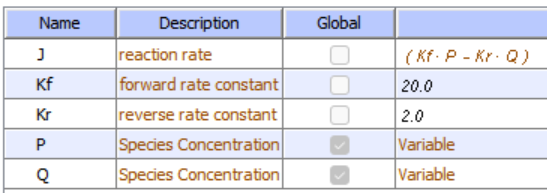
Now compare this same reaction, but in which S and P are part of the "mini-pathway" A ↔ S ↔ P ↔ Q, as shown in the Vcell model below. The enzyme kinetic parameters for S ↔ P (K_{M forward}, V_{M forward}, K_{M reverse}, V_{M reverse}) in the A ↔ S ↔ P ↔ O pathway were made the same as for the simple S ↔ P reaction, since it's the same enzyme. How do the A ↔ S and P ↔ Q reactions affect the apparent K_EQ? Run the Vcell model with the defaults automatically set to the values in the table above!

---

MODEL

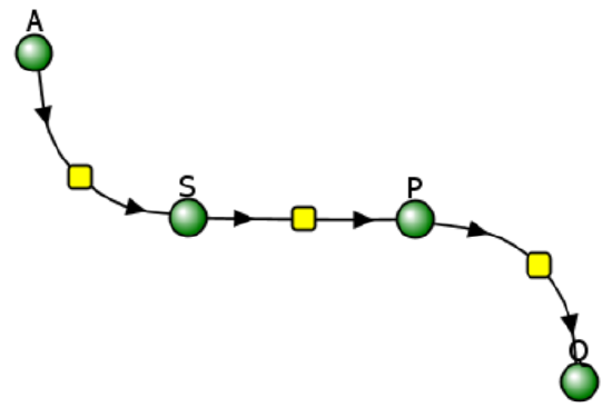
Initial Values

Select Load [model name] below

 Select Start to begin the simulation.

Interactive Element

Select Plot to change Y axis min/max, then Reset and Play  |  Select Slider to change which constants are displayed |  Select About  for software information.

Move the sliders to change the constants and see changes in the displayed graph in real-time.

Time course model made using Virtual Cell (Vcell), The Center for Cell Analysis & Modeling, at UConn Health.  Funded by NIH/NIGMS (R24 GM137787); Web simulation software (miniSidewinder) from Bartholomew Jardine and Herbert M. Sauro, University of Washington.  Funded by NIH/NIGMS (RO1-GM123032-04)

---

 

As in the first simulation, constant values for S and P are soon reached. Both are significantly lower than in the simple reaction of S ↔ P since P is being pulled toward Q faster than Q is converted back to S. Note also that Q reaches a higher concentration than either A or S, but remember that the sum of the initial values of A and S is 10.

Run the simulation again, but this time, set k_r=200 for the P ↔ Q reaction.

Now, calculate the "K_{EQ apparent}" for the different k_f values of the conversion of P → Q from this equation.  Again, use the CSV-downloaded spreadsheet data for each run you make.

\begin{equation}
K_{\text {eq apparent }}=\frac{[\mathrm{P}]_{\text {steady state }}}{[\mathrm{S}]_{\text {steady state }}}
\end{equation}

Do they equal 4 as in case 1? No, they do not! You should see that the "K_{EQ apparent}" value deviates most from 4 (lower number) when the rate constant for removal of P is highest (k_f=200).

Animations

Now, let's look at some animations of these reactions as an additional way to understand their dynamics. Click the image in Figure \(\PageIndex{4}\) to view (in a new window) the animation of the chemical species and an inserted graph showing concentration vs time for the reversible enzyme-catalyzed Reaction S ↔ P

Figure \(\PageIndex{4}\): Animation of the reversible enzyme-Catalyzed Reaction: S ↔ P

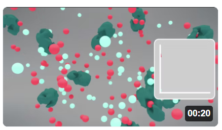
Pay attention to the disappearance of S (red) and the appearance of P (light blue) species after interacting with the enzyme (green).

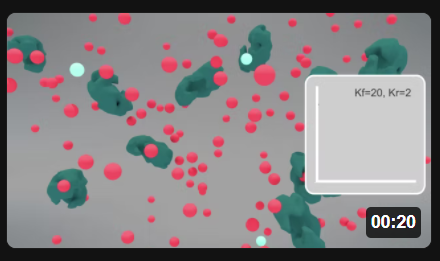
Now here are two animations for the S ↔ P reaction when it's embedded in the "minipathway" A ↔ S ↔ P ↔ Q, when k_f for the reaction P ↔ Q is 20 (left) and 200 (right). Click the images in Figure \(\PageIndex{5}\) to view (in a new window) an animation of the chemical species and inserted graphs showing concentrations vs time.

"mini-pathway" A ↔ S ↔ P ↔ Q, kf for the reaction P ↔ Q = 20	"mini-pathway" A ↔ S ↔ P ↔ Q, kf for the reaction P ↔ Q = 200

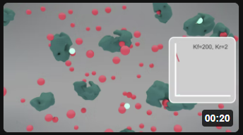Figure \(\PageIndex{5}\): Animation of the reversible enzyme-catalyzed Reaction embedded in a "minipathway" A ↔ S ↔ P ↔ Q when k_f for the reaction P ↔ Q is 200. S (red), P (light blue), and enzyme (green).

These animations should reinforce your understanding of the differences between equilibrium and steady-state conditions, although you can calculate the actual K_{EQ apparent} from the insert graphs without numerical data.

Understanding a pure enzyme in vitro and in vivo requires different approaches. Biochemists isolate and purify an enzyme found in some tissues and study its mechanism of action. When performing thermodynamic measurements to determine equilibrium constants (K_eq) or dissociation constants (K_D), from which ΔG⁰ can be calculated, a protein concentration is usually held constant as the binding ligand concentration is varied (independent variable). A dependent variable signal (often spectroscopic) is measured. Measurements are made when equilibrium is reached.

As we mentioned above (but it bears repeating), for enzyme kinetic measurements in vitro, the enzyme concentration is usually held constant as substrate and modifiers are varied (independent variables) to determine how velocity (dependent variable) changes. The substrate concentration determines the velocity. When inhibition is studied, the substrate concentration varies while the inhibitor concentration remains constant at several different fixed levels.

In vivo, the substrate concentration is determined by the reaction's velocity. For sets of reactions in pathways, flux (J) is used instead of velocity. In the steady state, the in and out fluxes for a given reaction are identical. Flux J is used to describe the rate of the system, whereas the rate or velocity v is used to describe the rate of an individual enzyme in a system.

Computer programs can find steady-state concentrations by finding the solution to the ordinary differential equations (ODE) when set to zero (v_f = v_r). To model a process at very low concentrations, programs can also use probabilistic or stochastic simulations to model probability distributions for species and their change with time for a finite number of particles. In such simulations, concentrations (in mM) are replaced with the number of particles/unit volume. ODEs don’t work well to describe these conditions since changes in concentrations are not continuous.

Now, let's return to our earlier rhetorical question of deriving the equations and determining all the relevant concentrations and constants for a pathway such as glycolysis. This has been done by Teusink et al. for glycolysis in yeast. Many complicated metabolic and signal transduction pathways have been mathematically modeled to understand cellular and organismal responses better. Quantitatively modeling and predicting concentrations, inputs, and outputs of all species in complex pathways is the basis of systems biology.

Basic Principles of Metabolic Control Analysis - Glycolysis

Let's use a more complex example, glycolysis, to illustrate the powers of computational modeling of entire pathways.  The reference for this model is shown below.

Can yeast glycolysis be understood in terms of the in vitro kinetics of the constituent enzymes? Testing biochemistry, Bas Teusink, Jutta Passarge, Corinne A. Reijenga, Eugenia Esgalhado, Coen C. van der Weijden, Mike Schepper, Michael C. Walsh, Barbara M. Bakker, Karel van Dam, Hans V. Westerhoff, and Jacky L. Snoep, 2000, European Journal of Biochemistry, 267, 5313-5329. PubMed ID: 10951190.  

Databases containing curated models with all the above information have been developed for many pathways. The yeast glycolysis model described in the reference above and the material below is found in the Biomodels Database. The model, BIOMD0000000064, can be downloaded as a Systems Biology Markup Language (SBML) file and imported into any of the programs described above. 

A variety of inputs are required for such computational analyses:

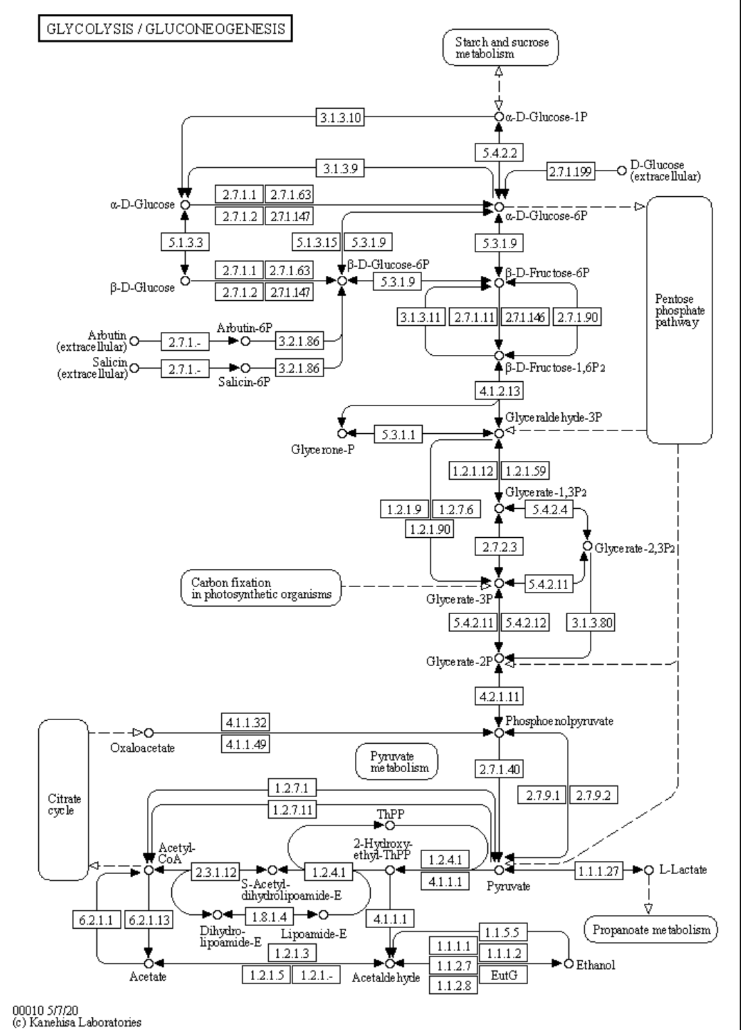
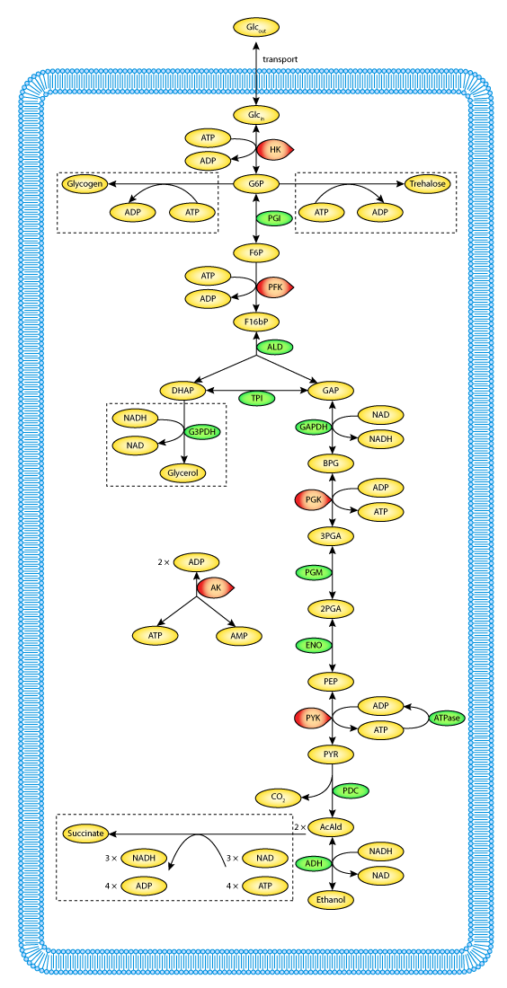
a. Defined pathways. These are available in many databases. An example from the KEGG pathways for yeast glycolysis is shown in the left panel of Figure \(\PageIndex{6}\) below. The right panel shows a more familiar representation, with glucose on the outside of the cell (Glc_o) entering the cell.

 

Figure \(\PageIndex{6}\): Left - Glycolysis Pathway from KEGG. http://www.genome.jp/dbget-bin/www_bget?pathway:sce00010;  Right - Teusink Glycolysis Model based on BIOMD0000000064.  https://models.physiomeproject.org/e/72/.  6:43am 23st April 2023.  CellML author(s): Catherine Lloyd.  Creative Commons Attribution 3.0 Unported License.

b. A computational modeling program to input all parameters, equations, and models and calculate concentrations for all species as a function of time. We have been using Vcell throughout this book. A reaction diagram is constructed that connects all the species involved.  Two are shown in Figure \(\PageIndex{7}\) below. 

Figure \(\PageIndex{7}\): Reaction Scheme for Yeast Glycolysis.  Left made using NEWT Pathway Viewer using Systems Biological Graphical Notation (SBGN) for BIOMD000000006.  Right is a reaction diagram using Vcell.  P represents ATP and ACE acetaldehyde.

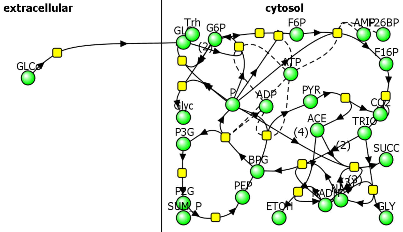The computational results from the analyses for yeast glycolysis were able to fit experimental data only if corrected by the addition of several branching reactions (shown in the figures above and Figure \(\PageIndex{8}\)) and in the dotted boxes in Figure 6 (Right)

Figure \(\PageIndex{8}\): Branching reactions for Yeast Glycolysis model (Teusink)

Trehalose is the non-reducing disaccharide Glc-(α 1,1)-Glc.  It is a reserve carbohydrate that also protects yeast against the effects of stress (desiccation, dehydration, temperature extremes) and lethal levels of ethanol.  These effects arise from its impact on protein stability, which is likely due to its preferential exclusion from the hydration sphere of proteins. A similar mechanism accounts for the stabilizing effect of glycerol on protein stability, as described in Chapter 4.9.

c. Table 2 below shows a list of all reactions as shown in Figure \(\PageIndex{10}\) for glycolysis and branching reactions (taken from COPASI).

Reaction	Name	Structure
ACE + NADH → NAD + ETOH	vADH	cytosol
F16P → 2TRIO	vALD	cytosol
P →	vATP	cytosol
P2G → PEP	vENO	cytosol
TRIO + NADH → NAD + GLY	vG3PDH	cytosol
NAD + TRIO → NADH + BPG	vGAPDH	cytosol
P + GLci → G6P	vGLK	cytosol
GLCo → GLci	vGLT	extracellular
G6P + P → Glyc	vGLYCO	cytosol
PYR → ACE + CO2	vPDC	cytosol
P + F6P → F16P	vPFK	cytosol
G6P → F6P	vPGI	cytosol
BPG → P + P3G	vPGK	cytosol
P3G → P2G	vPGM	cytosol
PEP → P + PYR	vPYK	cytosol
3NAD + 4P + 2ACE → 3NADH + SUCC	vSUC	cytosol
2G6P + P → Trh	vTreha	cytosol

Table  \(\PageIndex{2}\): List of reactants and concentrations for yeast glycolysis.  P is ATP, ACE is acetaldehyde, a reactant/product of the enzyme alcohol dehydrogenase.

 

d. Parameters (concentrations, rate, enzyme kinetics, and equilibrium constants) of all species. Table \(\PageIndex{3}\) below shows the initial concentrations for the glycolysis model. 

Species	Structure	Clamped	Conc (mM)
GLCo	extracellular	TRUE	50
GLCi	cytosol	FALSE	0.087
G6P	cytosol	FALSE	2.45
F6P	cytosol	FALSE	0.62
F16P	cytosol	FALSE	5.51
TRIO	cytosol	FALSE	0.96
BPG	cytosol	FALSE	0
P3G	cytosol	FALSE	0.9
P2G	cytosol	FALSE	0.12
PEP	cytosol	FALSE	0.07
PYR	cytosol	FALSE	1.85
ACE	cytosol	FALSE	0.17
P	cytosol	FALSE	6.31
NAD	cytosol	FALSE	1.2
NADH	cytosol	FALSE	0.39
Glyc	cytosol	TRUE	0
Trh	cytosol	TRUE	0
CO2	cytosol	TRUE	1

Table  \(\PageIndex{3}\):  Initial concentrations for the glycolysis model. Clamped TRUE means concentrations were fixed.

 

e. Equations that can be used to compute the change in concentrations of all species with time. These are usually ordinary differential equations (ODEs) as described in Chapter 6B - Kinetics of Simple and Enzyme-Catalyzed Reactions, Sections B1: Single Step Reactions.) ODEs are easy to write but require a computer to solve as the number of interacting species increases.

For a quick review, consider the relatively simple reaction scheme shown in Figure \(\PageIndex{12}\) below. The set of ODEs for each species is shown below.

Figure \(\PageIndex{12}\): Chemical reactions for ODEs

This set of ODEs for each species can be written.

\begin{equation}
\begin{aligned}
\frac{d[A]}{d t} &=-k_1[A][B]+k_2[C] \\
\frac{d[B]}{d t} &=-k_1[A][B]+k_2[C] \\
\frac{d[C]}{d t} &=+k_1[A][B]-k_2[C]-k_3[C]=+k_1[A][B]-\left(k_2+k_3\right)[C] \\
\frac{d[D]}{d t} &=+k_3[C]
\end{aligned}
\end{equation}

If a reaction removes species X, the right side of the ODE for the disappearance of that species has a – sign for that term. Likewise, if a reaction increases the concentration of species X, the right-hand side has a positive sign. The above examples illustrate unimolecular (C to D, C to A + B) and bimolecular (A + B to C) reactions.

Now, let's examine the equations specifically for the change in the concentration of glucose-6-phosphate. Two reactions can form it, and four reactions can remove it (check arrows for reversibility), as shown in Figure \(\PageIndex{13}\) below.

Figure \(\PageIndex{13}\): The reactions that change [G6P] in the Teusink yeast glycolysis model

An ODE can be written for the change in the concentration of glucose-6-phosphate.

\begin{equation}
\left.\mathrm{d}[\mathrm{G} 6 P] / \mathrm{dt}=v_{\mathrm{HK}}-v_{\mathrm{PGI}}-2 v_{\text {trehalose }}-v_{\text {glycogen }}\right)
\end{equation}

where HK is hexokinase and PGI is phosphoglucoisomerase. Note their is a coefficient of 2 for the formation of trehalose since it takes 2 G6Ps to make 1 trehalose.

Let's look at the terms and how they are written in Vcell.

Formation of G6P

Only one reaction goes towards G6P.  It's the reaction catalyzed by hexokinase (G + ATP →  G6P + ADP).  In the Vcell reaction diagram, ATP is represented by P.  Flux J =

\begin{equation}
\frac{V m G L K \cdot\left(G L C i \cdot A T P-\frac{G 6 P \cdot A D P}{K e q G L K}\right)}{K m G L K G L C i \cdot K m G L K A T P \cdot\left(1.0+\frac{G L C i}{K m G L K G L C i}+\frac{G 6 P}{K m G L K G 6 P}\right) \cdot\left(1.0+\frac{A T P}{K m G L K A T P}+\frac{A D P}{K m G L K A D P}\right)}
\end{equation}

Removal of G6P

3 reactions go away from G6P.

i.  G6P → F6P.    Flux J =

\begin{equation}
\frac{V m P G I_{-} 2 \cdot\left(G 6 P-\frac{F 6 P}{K e q P G I_{-} 2}\right)}{K m P G I G 6 P_{-} 2 \cdot\left(1.0+\frac{G 6 P}{K m P G I G 6 P \_2}+\frac{F 6 P}{K m P G I F 6 P_{-}2}\right)}
\end{equation}

ii.  G6P → Glycogen

Flux J = KGLYCOGEN_3

iii.  G6P → Trehalose

Flux J = KTREHALOSE

Now let's run a simulation of the model of yeast glycolysis (Teusink,B et al.: Eur J Biochem 2000 Sep;267(17):5313-29).  The actual model is available from Biomodels (BIOMD0000000064). 

Yeast Glycolysis

Yeast Glycolysis

Teusink et al., 2000.  BIOMD0000000064

 

 

 

For Figure \(\PageIndex{14}\) below, the model was run, and the CSV file was used to plot the concentration vs time plots for each species.  Two species, EtOH (50 mM) and GLCo - glucose outside (50 mM), have fixed concentrations much larger than the rest, so they are omitted from the graph for clarity. When you run the simulation above, repeat the process by downloading the CSV file and plotting the progress curves.  Also, note that the y-axis values are not shown correctly when you run the simulation.  Rescale them in the spreadsheet based on the correct values of EtOH and GLC0, which were held constant (clamped) throughout the time course at 50 mM.  

Figure \(\PageIndex{14}\): Time course graphs of all glycolytic species vs time

How closely does simulation replicate fluxes found experimentally in vivo?  As mentioned above, without the addition of the branch reaction, a steady state was not achieved in the simulation. Fluxes in the model were within a factor of two for only about half of the enzymes, indicating that the model requires improvement.  Other discrepancies could be attributed to differences in kinetics in vivo compared to in vitro measurements.  Additional products (glycogen, trehalose, glycerol, and succinate) were derived from glucose, which mainly entered glycolysis and was converted to ethanol, highlighting the complexity of modeling even a relatively "simple" pathway like glycolysis.

Metabolic Control Analysis and Simple Enzyme Inhibition

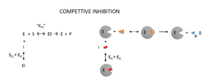
Biochemists model complex enzyme-catalyzed reactions in the presence and absence of modifiers (either activators or inhibitors) to develop reaction mechanisms. The following kinetic parameters are experimentally determined by fitting the initial velocity (vo) vs substrate concentration ([S]) through nonlinear fitting algorithms.

• K_m – the Michaelis Constant, the concentration of substrate at half-maximal velocity;
• V_m – the velocity at saturating substrate concentration;
• k_cat - the turnover number for conversion of bound reactant to product;
• K_ix – inhibition dissociation constants.

An example of competitive inhibition, shown in Figure \(\PageIndex{15}\), illustrates a common type of analysis for such reactions.

Figure \(\PageIndex{15}\): Chemical reactions for competitive inhibition

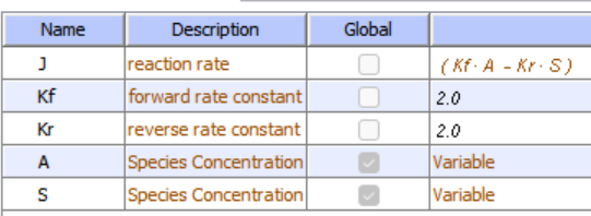
One modern pictorial depiction of a simple irreversible, enzyme-catalyzed reaction of substrate S going to product P with inhibition by the product and by an added inhibitor is shown in Figure \(\PageIndex{16}\). The square, a "node" in the reaction diagram, represents the enzyme.

Figure \(\PageIndex{16}\): Pictorial Description for product and separate competitive inhibitor

Consider the simple enzyme-catalyzed reaction for a reversible conversion of substrate S to product P that has three reversible steps, as shown in Figure \(\PageIndex{17}\)

Figure \(\PageIndex{17}\): Three step reversible enzyme-catalyzed reaction

If the forward (f) and reverse (r) chemical reaction steps were irreversible and written separately, simple Michaelis-Menten equations could be written for each.

\begin{equation}
\begin{aligned}
&v_f=\frac{V_f S}{K_{M S}+S}=\frac{\frac{V_f S}{K_{M S}}}{1+\frac{S}{K_{M S}}} \\
&v_r=\frac{V_r P}{K_{M P}+P}=\frac{\frac{V_r P}{K_{M P}}}{1+\frac{P}{K_{M P}}}
\end{aligned}
\end{equation}

For the actual reversible reactions, the net forward rate cannot be found by simple subtraction of the two equations above as the differential equations describing the simple forward and reverse rates don’t account for the reverse steps

\begin{equation}
v \neq\left[\frac{\frac{V_f S}{K_{M S}}}{1+\frac{S}{K_{M S}}}-\frac{\frac{V_r P}{K_{M P}}}{1+\frac{P}{K_{M P}}}\right]
\end{equation}

A simple derivation (assuming rapid equilibrium for both forward and reverse steps) can be made for the net forward reaction. Again, consider the following enzyme-catalyzed reaction (Figure 17 above):

A derivation of the rapid equilibrium, fully reversible Michaelis-Menten equation conversion of substrate S to product P

Here it is if you wish to see it!

Derivation

You may remember that for the isolated E + S ↔ ES and for the E + P ↔ EP reactions, the simple dissociation constants, K_S and K_P are given by

\begin{equation}
\begin{aligned}
&K_S=\frac{E_{e q} S_{e q}}{E S_{e q}}=\frac{k_{-1}}{k_1} \text { or } E S=\frac{[E][S]}{K_S} \\
&K_P=\frac{E_{e q} P_{e q}}{E P_{e q}}=\frac{k_3}{k_{-3}} \text { or } E P=\frac{[E][P]}{K_P}
\end{aligned}
\end{equation}

The rapid equilibrium assumption states that the rate of dissociation of ES and EP, which are both physical steps, is much faster than the rate of the chemical conversion steps for each complex. Hence, \(k_{-1} \gg k_2\) and \(k_3 \gg k_{-2}\), so the relative amounts of ES and EP can be determined from the dissociation constants as shown above.

Mass conservation of enzymes gives

\begin{equation}
E_0=E+E S+E P=E+\frac{[E][S]}{K_S}+\frac{[E][P]}{K_p}=E\left[1+\frac{[S]}{K_S}+\frac{[P]}{K_p}\right]
\end{equation}

From this, we can get the fractional amount of both ES and EP

\begin{equation}
\begin{aligned}
&\frac{E S}{E_0}=\frac{\frac{[E][S]}{K_S}}{E\left[1+\frac{[S]}{K_S}+\frac{[P]}{K_p}\right]} \text { or } E S=\frac{E_0 \frac{[S]}{K_S}}{\left[1+\frac{[S]}{K_S}+\frac{[P]}{K_p}\right]} \\
&\frac{E P}{E_0}=\frac{[E][P]}{E\left[1+\frac{[S]}{K_S}+\frac{[P]}{K_P}\right]} \text { or } E P=\frac{E_0 \frac{[P]}{K_P}}{\left[1+\frac{[S]}{K_S}+\frac{[P]}{K_P}\right]}
\end{aligned}
\end{equation}

Now, we can derive the rate equation for the net forward reaction for the rapid equilibrium case:

\begin{equation}
v=k_2[E S]-k_{-2}[E P]=k_2 \frac{E_0 \frac{[S]}{K_S}}{\left[1+\frac{[S]}{K_S}+\frac{[P]}{K_p}\right]}-k_{-2} \frac{E_0 \frac{[P]}{K_p}}{\left[1+\frac{[S]}{K_S}+\frac{[P]}{K_p}\right]}
\end{equation}

Knowing that k₂E₀ and k_-2E₀ represent the maximal velocities, V_f and V_r, respectively, the equation becomes:

\begin{equation}
v=k_2[E S]-k_{-2}[E P]=\frac{V_f \frac{[S]}{K_S}}{\left[1+\frac{[S]}{K_S}+\frac{[P]}{K_p}\right]}-\frac{V_r \frac{[P]}{K_p}}{\left[1+\frac{[S]}{K_S}+\frac{[P]}{K_p}\right]}=\frac{V_f \frac{[S]}{K_S}-V_r \frac{[P]}{K_p}}{\left[1+\frac{[S]}{K_S}+\frac{[P]}{K_p}\right]}
\end{equation}

 

Here is the derived equation.

\begin{equation}
v=k_2[E S]-k_{-2}[E P]=\frac{V_f \frac{[S]}{K_S}}{\left[1+\frac{[S]}{K_S}+\frac{[P]}{K_p}\right]}-\frac{V_r \frac{[P]}{K_p}}{\left[1+\frac{[S]}{K_S}+\frac{[P]}{K_p}\right]}=\frac{V_f \frac{[S]}{K_S}-V_r \frac{[P]}{K_p}}{\left[1+\frac{[S]}{K_S}+\frac{[P]}{K_p}\right]}
\end{equation}

An equation of a similar form can be derived from the steady state assumption. Hence, the net forward rate can't be determined by the simple subtraction of the backward rate from the forward rate, as shown in Equation 10 above. 

Common Forms of Kinetic Equations

Programs like COPASI and VCell have many built-in equations for the velocities of many enzyme-catalyzed reactions with similar forms. Two are shown below:

Reversible Michaelis-Menten:

\begin{equation}
\frac{\frac{V_f[\text { substrate }]}{K_{M s}}-\frac{V_r[\text { product }]}{K_{M p}}}{1+\frac{[\text { substrate }]}{K_{M s}}+\frac{[\text { product }]}{K_{M p}}}
\end{equation}

Competitive Inhibition Reversible:

\begin{equation}
\frac{\frac{V_f[\text { substrate }]}{K_{M s}}-\frac{V_r[\text { product }]}{K_{M p}}}{1+\frac{[\text { substrate }]}{K_{M s}}+\frac{[\text { product }]}{K_{M p}}+\frac{[\text { inhibitor }]}{K_I}}
\end{equation}

What is most important for readers to understand is not detailed derivations or how to solve the differential equations on their own. However, you should be able to:

• write the differential equation of a given reaction.
• recognize the common equations used for nonenzyme-catalyzed reactions (mass action) and enzyme-catalyzed ones;
• change parameters in programs that use numerical methods to solve systems of linked differential equations for a system, and see how the time course graphs are affected.

Summary

This chapter introduces the fundamentals of metabolic control analysis (MCA) by exploring the complexities of enzyme kinetics within metabolic pathways. It begins by addressing the challenges inherent in studying enzyme-catalyzed reactions, including the involvement of multiple chemical species, numerous rate and dissociation constants, and complex reaction mechanisms. Key highlights include:

• Complexity in Enzyme Kinetics:
  The chapter outlines the difficulties in deriving kinetic equations for enzyme-catalyzed reactions, using an example that demonstrates how multiple reaction steps and intermediates can be mathematically described by ordinary differential equations (ODEs).

• Equilibrium vs. Steady State:
  Two scenarios are contrasted: a closed system reaching equilibrium (with no net change in reactant or product concentrations) and an open system achieving a steady state where inputs equal outputs. The steady state concept is emphasized as more relevant to in vivo conditions, where enzymes operate under continuous flux rather than static equilibrium.

• In Vitro vs. In Vivo Kinetics:
  A significant portion of the chapter is devoted to understanding the differences between controlled laboratory experiments (in vitro) and the dynamic environment of the cell (in vivo). The discussion highlights that while in vitro assays focus on initial rate measurements with varying substrate concentrations, in vivo systems are governed by steady-state fluxes that maintain balanced metabolite levels.

• Simulation and Modeling Tools:
  The use of computational tools like VCell and COPASI is introduced to simulate progress curves (concentration versus time) for enzyme reactions. These simulations illustrate how embedding an enzyme within a “mini-pathway” alters its apparent equilibrium constant compared to when it is studied in isolation.

• Derivation of Kinetic Equations:
  The chapter walks through the derivation of a net forward rate equation for reversible enzyme reactions under rapid equilibrium assumptions. It explains why the net rate cannot simply be determined by subtracting the reverse rate from the forward rate, and extends the discussion to include the impact of enzyme inhibitors.

• Modeling Complex Pathways:
  Using yeast glycolysis as a model system, the chapter demonstrates how complex pathways are mathematically modeled. It covers the integration of branching reactions, parameterization with experimental data, and the construction of reaction schemes to account for the dynamic behavior of metabolites.

Overall, this chapter equips students with both the theoretical framework and practical skills necessary for analyzing and modeling metabolic networks. By combining mathematical derivations with computational simulations, junior and senior biochemistry majors gain a comprehensive understanding of how enzyme kinetics and pathway dynamics are integrated within the broader context of systems biology.