14.2: Population Growth and Regulation

Although life histories describe the way many characteristics of a population (such as their age structure) change over time in a general way, population ecologists make use of a variety of methods to model population dynamics mathematically. These more precise models can then be used to accurately describe changes occurring in a population and better predict future changes. Certain models that have been accepted for decades are now being modified or even abandoned due to their lack of predictive ability, and scholars strive to create effective new models.

Population ecologists make use of a variety of methods to model population dynamics. An accurate model should be able to describe the changes occurring in a population and predict future changes. The two simplest models of population growth use deterministic equations (equations that do not account for random events) to describe the rate of change in the size of a population over time (Figure \(\PageIndex{1}\)). The first of these models, exponential growth, describes populations that increase in numbers without any limits to their growth. The second model, logistic growth, introduces limits to reproductive growth that become more intense as the population size increases. Neither model adequately describes natural populations, but they provide points of comparison.

 

Figure \(\PageIndex{1}\): When resources are unlimited, populations exhibit exponential growth, resulting in a J-shaped curve. When resources are limited, populations exhibit logistic growth. In logistic growth, population expansion decreases as resources become scarce, and it levels off when the carrying capacity of the environment is reached, resulting in an S-shaped curve.

The Population Growth Rate (r )

The population growth rate (sometimes called the rate of increase or per capita growth rate, r) equals the birth rate (b) minus the death rate (d) divided by the initial population size (N₀).

Another method of calculating the population growth rate involves final and initial population size (figure \(\PageIndex{2}\)). In this case, population growth rate (r) equals the final population size (N) minus the initial population size (N₀) and divided by the initial population size (N₀).

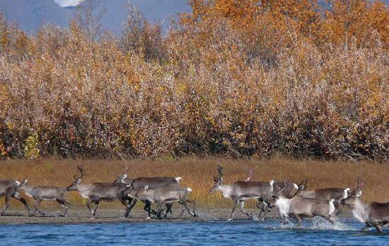
Figure \(\PageIndex{2}\): How could we calculate the growth rate of this caribou population per year if there were 200 individuals in 2016 and 300 individuals in 2018? Image by K. Joly/NPS (public domain).

Exponential Growth

Charles Darwin, in his theory of natural selection, was greatly influenced by the English clergyman Thomas Malthus. Malthus published a book in 1798 stating that populations with unlimited natural resources grow very rapidly, and then population growth decreases as resources become depleted. This accelerating pattern of increasing population size is called exponential growth. 

The best example of exponential growth is seen in bacteria. Bacteria are prokaryotes that reproduce quickly, about an hour for many species.  If 1000 bacteria are placed in a large flask with an unlimited supply of nutrients (so the nutrients will not become depleted), after an hour, there is one round of division and each organism divides, resulting in 2000 organisms—an increase of 1000 (Figure \(\PageIndex{3}\)). In another hour, each of the 2000 organisms will double, producing 4000, an increase of 2000 organisms. After the third hour, there should be 8000 bacteria in the flask, an increase of 4000 organisms. The important concept of exponential growth is that the population growth rate—the number of organisms added in each reproductive generation—is accelerating; that is, it is increasing at a greater and greater rate. After 1 day and 24 of these cycles, the population would have increased from 1000 to more than 16 billion. When the population size, N, is plotted over time, a J-shaped growth curve is produced (Figure \(\PageIndex{1}\)).

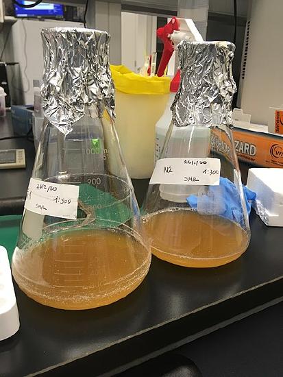
Figure \(\PageIndex{3}\): Bacteria growing with abundant nutrients in a flask will exhibit exponential growth. Image by Soledad Mirand-Rottman (CC-BY-SA).

The bacteria-in-a-flask example is not truly representative of the real world where resources are usually limited. However, when a species is introduced into a new habitat that it finds suitable, it may show exponential growth for a while. In the case of the bacteria in the flask, some bacteria will die during the experiment and thus not reproduce; therefore, the growth rate is lowered from a maximal rate in which there is no mortality.  Additionally, ecologists are interested in the population at a particular point in time, an infinitely small time interval. For this reason, the terminology of differential calculus is used to obtain the “instantaneous” growth rate, replacing the change in number and time with an instant-specific measurement of number and time.

\[\frac{d N} {d T} = bN - dN = (b - d)N \nonumber\]

Notice that the “d” associated with the first term refers to the derivative (as the term is used in calculus) and is different from the death rate, also called “\(d\).” The difference between birth and death rates is further simplified by substituting the term “r” (intrinsic rate of increase) for the relationship between birth and death rates:

\[\frac{d N} {d T} = rN \nonumber\]

The value “\(r\)” can be positive, meaning the population is increasing in size; or negative, meaning the population is decreasing in size; or zero, where the population’s size is unchanging, a condition known as zero population growth. A further refinement of the formula recognizes that different species have inherent differences in their intrinsic rate of increase (often thought of as the potential for reproduction), even under ideal conditions. Obviously, a bacterium can reproduce more rapidly and have a higher intrinsic rate of growth than a human. The maximal growth rate for a species is its biotic potential, or \(r_{max}\), thus changing the equation to:

\[\frac{d N} {d T} = r_\text{max}N \nonumber\]

Populations of all species can, potentially, increase rapidly under conditions in which resource availability and other factors are not constraining. Examples of rapid population growth are illustrated in Figure \(\PageIndex{4}\). However, unlimited growth cannot be sustained – in all of the cases in Figure \(\PageIndex{4}\), the population sizes eventually leveled off, decreased, or crashed.

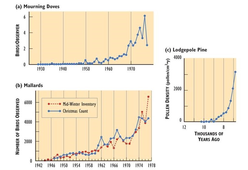
Figure \(\PageIndex{4}\): Rapid Growth of Some Natural Populations. (a) The population of mourning doves (Zenaida macroura) wintering in southern Ontario over 48 years. This used to be a rare bird, but it has apparently benefited from a warming climate, suburban habitat, and winter feeding. (b) The population of mallards (Anas platyrhynchos) wintering in southern Ontario over 35 years, illustrated with two independent sets of data. This duck has expanded its breeding and wintering ranges into eastern Canada, likely in response to habitat made available by the clearing of forest. (c) The population of lodgepole pine (Pinus contorta) near Snowshoe Lake, British Columbia, during natural afforestation following deglaciation 7000-9000 years ago. In this case, tree populations are indicated by the amount of pollen in dated layers of lake sediment. Sources: Modified from (a) Freedman and Riley (1980); (b) Goodwin et al. (1977); (c) MacDonald and Cwynar (1991).

Logistic Growth

Exponential growth is possible only when infinite natural resources are available; this is not the case in the real world. Charles Darwin recognized this fact in his description of the “struggle for existence,” which states that individuals will compete (with members of their own or other species) for limited resources. The successful ones will survive to pass on their own characteristics and traits (which we know now are transferred by genes) to the next generation at a greater rate (natural selection). To model the reality of limited resources, population ecologists developed the logistic growth model.

In the real world, with its limited resources, exponential growth cannot continue indefinitely. Exponential growth may occur in environments where there are few individuals and plentiful resources, but when the number of individuals gets large enough, resources will be depleted, slowing the growth rate. Eventually, the growth rate will plateau or level off (Figure \(\PageIndex{1 and 4}\)). This population size, which represents the maximum population size that a particular environment can support, is called the carrying capacity, or \(K\).  There are three different sections to an S-shaped curve. Initially, growth is exponential because there are few individuals and ample resources available. Then, as resources begin to become limited, the growth rate decreases. Finally, growth levels off at the carrying capacity of the environment, with little change in population size over time.

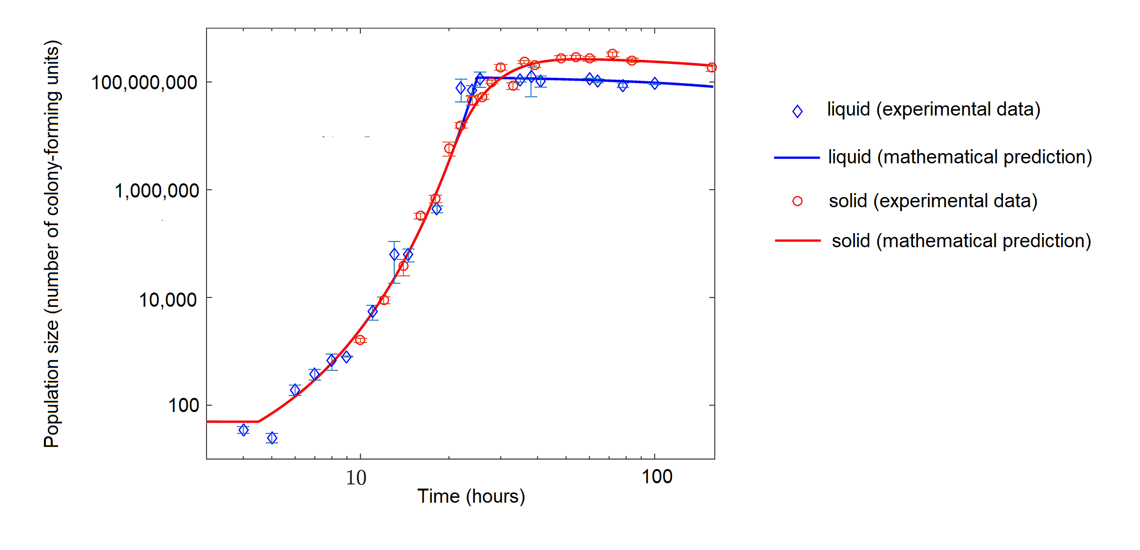
Figure \(\PageIndex{4}\): The growth of the bacterium Escherichia coli (E. coli) with limited nutrients over time in hours. Population size is in number of colony-forming units, which is a cell capable of dividing to produce a colony of cells. The bacteria were grown in liquid (blue diamonds) or on a semisolid medium (agar, red circles). The points represent actual measurements of populations size, and the lines represent a mathematical model, basically a prediction that is based on the data points. The data show logistic population growth, particularly in solid media. Initially, population size increases rapidly (concave part of curve), but the growth rate then stabilizes (straight line) before decreasing (convex part of curve) and leveling near the carrying capacity. Image modified from Shao X, Mugler A, Kim J, Jeong HJ, Levin BR, Nemenman I (2017) Growth of bacteria in 3-d colonies. PLoS Comput Biol 13(7): e1005679 (CC-BY).

In some populations, there are variations to the S-shaped curve. Examples in wild populations include sheep and harbor seals (figure \(\PageIndex{5}\)). In both examples, the population size exceeds the carrying capacity for short periods of time and then falls below the carrying capacity afterwards. This fluctuation in population size continues to occur as the population oscillates around its carrying capacity. Still, even with this oscillation the logistic model is confirmed.

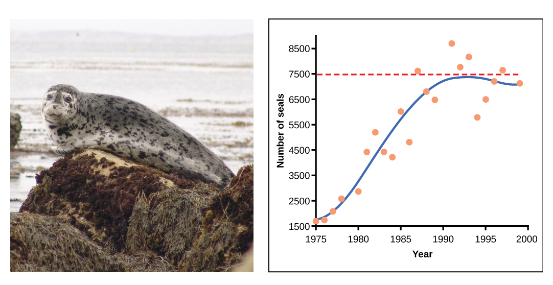
Figure \(\PageIndex{5}\): A natural population of seals shows logistic growth. The number of seals, ranging from 1500 to 8500, is on the y-axis, and the year, ranging from 1975-2000, is on the x-axis. Orange dots represent the observed population size each year, and the blue line represent the trend. From 1975 to 1983, the blue line curves upwards, representing an increase in both population size and population growth rate. From 1983 to 1992, the curve flattens, representing that population size is still increasing, but population growth rate is decreasing. After 1992, population fluctuates near the carrying capacity (dotted, horizontal line). 

The formula we use to calculate logistic growth adds the carrying capacity as a moderating force in the growth rate. The expression “\(K – N\)” is indicative of how many individuals may be added to a population at a given stage, and “\(K – N\)” divided by “\(K\)” is the fraction of the carrying capacity available for further growth. Thus, the exponential growth model is restricted by this factor to generate the logistic growth equation:

\[\begin{align} \dfrac{d N} {d T}
&= r_\text{max} \frac{d N} {d T} \nonumber \\[5pt]
&= r_\text{max}N \frac{(K-N)} {K}\nonumber
\end{align} \nonumber\]

Notice that when \(N\) is very small, \((K-N)/K\) becomes close to \(K/K\) or \(1\), and the right side of the equation reduces to \(r_{max}N\), which means the population is growing exponentially and is not influenced by carrying capacity. On the other hand, when \(N\) is large, \((K-N)/K\) come close to zero, which means that population growth will be slowed greatly or even stopped. Thus, population growth is greatly slowed in large populations by the carrying capacity \(K\). This model also allows for the population of a negative population growth, or a population decline. This occurs when the number of individuals in the population exceeds the carrying capacity (because the value of \((K-N)/K\) is negative).

The logistic model assumes that every individual within a population will have equal access to resources and, thus, an equal chance for survival. For plants, the amount of water, sunlight, nutrients, and the space to grow are the important resources, whereas in animals, important resources include food, water, shelter, nesting space, and mates.  In the real world, phenotypic variation among individuals within a population means that some individuals will be better adapted to their environment than others. The resulting competition between population members of the same species for resources is termed intraspecific competition (intra- = “within”; -specific = “species”). Intraspecific competition for resources may not affect populations that are well below their carrying capacity—resources are plentiful and all individuals can obtain what they need. However, as population size increases, this competition intensifies. In addition, the accumulation of waste products can reduce an environment’s carrying capacity.  

The logistic population growth model is not the only way that populations respond to limited resources. In some populations, growth is exponential until resources run low, wastes accumulate, or disease spreads (see limiting factors below), and the population then crashes (Figure \(\PageIndex{5}\)). Thus, population growth rate (and size) may plummet rapidly instead of tapering as it approaches the carrying capacity. 

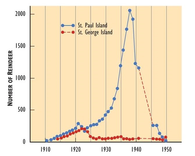
Figure \(\PageIndex{5}\):  Population Growth and Crash. In 1910, reindeer (Rangifer tarandus tarandus; the Eurasian subspecies of caribou) were introduced to two islands in the Aleutian chain off Alaska in an attempt to establish a new food resource for local use. On both islands, the reindeer population increased rapidly. However, they exceeded the carrying capacity of the habitat and caused severe damage through overgrazing. The populations then crashed. Source: Modified from Krebs (1985).

Factors that Regulate Population Growth

The logistic model of population growth, while valid in many natural populations and a useful model, is a simplification of real-world population dynamics. Implicit in the model is that the carrying capacity of the environment does not change, which is not the case. The carrying capacity varies annually: for example, some summers are hot and dry whereas others are cold and wet. In many areas, the carrying capacity during the winter is much lower than it is during the summer. Also, natural events such as earthquakes, volcanoes, and fires can alter an environment and hence its carrying capacity. Additionally, populations do not usually exist in isolation. They engage in interspecific competition: that is, they share the environment with other species, competing with them for the same resources. These factors are also important to understanding how a specific population will grow.

Nature regulates population growth in a variety of ways. These are grouped into density-dependent factors, in which the density of the population at a given time affects growth rate and mortality, and density-independent factors, which influence mortality in a population regardless of population density. Note that in the former, the effect of the factor on the population depends on the density of the population at onset. Conservation biologists want to understand both types because this helps them manage populations and prevent extinction or overpopulation.

Density-dependent Regulation

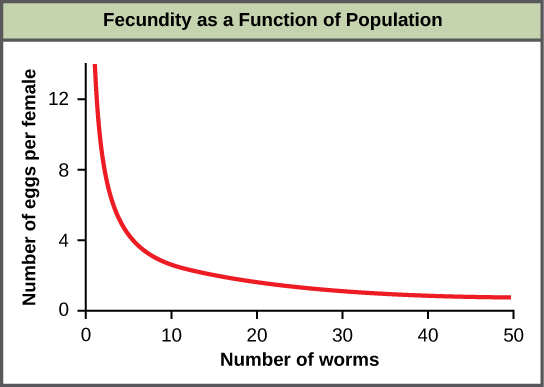
Most density-dependent factors are biological in nature (biotic). Usually, the denser a population is, the greater its mortality rate. Density-dependent factors include predation, parasitism, herbivory, competition, and accumulation of waste. An example of density-dependent regulation is shown in figure \(\PageIndex{6}\) with results from a study focusing on the giant intestinal roundworm (Ascaris lumbricoides), a parasite of humans and other mammals. Denser populations of the parasite exhibited lower fecundity: they contained fewer eggs. One possible explanation for this is that females would be smaller in more dense populations (due to limited resources) and that smaller females would have fewer eggs. This hypothesis was tested and disproved in a 2009 study which showed that female weight had no influence. The actual cause of the density-dependence of fecundity in this organism is still unclear and awaiting further investigation.

Figure \(\PageIndex{6}\): In this population of roundworms, fecundity (number of eggs) decreases with population density.³

As a population increases, its predators are able to harvest it more easily. Prey density also affects population growth rate of predators: low prey density increases the mortality of its predator because it has more difficulty locating its food sources.  Parasites are able to pass from host to host more easily as the population density of the host increases. For this reason, epidemics among humans are particularly severe in cities. In fact, for most of the period since humans began living in cities, city populations have been maintained only through continual immigration from the countryside. Not until the development of community sanitation, immunization, and other public health measures did cities avoid periodic sharp drops in population as a result of epidemics. The recurrent epidemics of the "black death" in Europe that began in the fourteenth century caused a sharp decline in population. In just three years (1348–1350), at least one-quarter of the population of Europe died from the disease (probably plague). Similarly, herbivores can more easily spread between individual plants in a dense population. This is why strip cropping helps control pests. An herbivore or plant pathogen may infect one row of plants, but it is less likely to spread to more distant rows of that species.

Intraspecific competition (and interspecific competition) can be important density dependent factors. In the summer of 1980, much of southern New England was struck by an infestation of the gypsy moth (figure \(\PageIndex{6}\)). As the summer wore on, the larvae (caterpillars) pupated, the hatched adults mated, the females laid masses of eggs (each mass containing several hundred eggs) on virtually every tree in the region. In early May of 1981, the young caterpillars that hatched from these eggs began feeding and molting.  In 72 hours, a 50-ft beech tree or a 25-ft white pine tree would be completely defoliated. Large patches of forest began to take on a winter appearance with their skeletons of bare branches. In fact, the infestation was so heavy that many trees were completely defoliated before the caterpillars could complete their larval development. The result: a massive die-off of the animals; very few succeeded in completing metamorphosis. Here, then, was a dramatic example of how competition among members of one species for a finite resource - in this case, food - caused a sharp drop in population. The effect was clearly density-dependent. The lower population densities of the previous summer had permitted most of the animals to complete their life cycle.

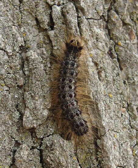
Figure \(\PageIndex{6}\): Gypsy moth caterpillars face intraspecific competition at high densities. Image by Editor at Large (CC-BY-SA).  

Density-independent Regulation

Many factors, typically physical or chemical in nature (abiotic), influence the mortality of a population regardless of its density, including weather, natural disasters, and pollution (Figure \(\PageIndex{7}\)). An individual deer may be killed in a forest fire regardless of how many deer happen to be in that area. Its chances of survival are the same whether the population density is high or low. The same holds true for cold winter weather.  Not only do abiotic factors limit population growth but they often drive existing populations well below their previous level.

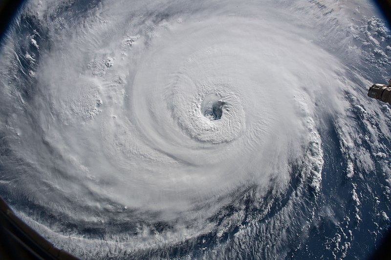
Figure \(\PageIndex{7}\): Severe weather, like Hurricane Florence of 2018, can reduce population size regardless of density. Image by NASA Goddard Space Flight Center (CC-BY)

These factors are described as density-independent because they exert their effect irrespective of the size of the population when the catastrophe struck.  This graph (Figure \(\PageIndex{8}\), from P. T. Boag and P.R. Grant in Science, 214:82, 1981) shows the decline in the population of one of Darwin's finches (Geospiza fortis) on Daphne Major, a tiny (100 acres = 40 hectares) member of the Galapagos Islands. The decline (from 1400 to 200 individuals) occurred because of a severe drought that reduced the quantity of seeds on which this species feeds. The drought ended in 1978, but even with ample food once again available the finch population recovered only slowly.

Figure \(\PageIndex{7}\): Left: This graph (from P. T. Boag and P.R. Grant in Science, 214:82, 1981) shows the decline in the population of one of Darwin's finches (Geospiza fortis) on Daphne Major, a tiny (100 acres = 40 hectares) member of the Galapagos Islands. The decline (from 1400 to 200 individuals) occurred because of a severe drought that reduced the quantity of seeds on which this species feeds.  Right: The graph (redrawn from R. H. MacArthur and E. O. Wilson, The Theory of Island Biogeography, Princeton University Press) shows the number of species of reptiles and amphibians on various islands in the West Indies.

In real-life situations, population regulation is very complicated and density-dependent and independent factors can interact. A dense population that is reduced in a density-independent manner by some environmental factor(s) will be able to recover differently than a sparse population. For example, a population of deer affected by a harsh winter will recover faster if there are more deer remaining to reproduce.

Catastrophic declines are particularly risky for populations living on islands. The smaller the island, the smaller the population of each species on it, and the greater the risk that a catastrophe will so decimate the population that it becomes extinct. This appears to be one reason for the clear relationship between size of island and the number of different species it contains.  The graph (Figure \(\PageIndex{8}\), redrawn from R. H. MacArthur and E. O. Wilson, The Theory of Island Biogeography, Princeton University Press) shows the number of species of reptiles and amphibians on various islands in the West Indies. In general, if one island has 10 times the area of another, it will contain approximately twice the number of species.  The same principle applies to many habitats. In a sense, most habitats are islands. A series of ponds, a range of mountain tops, scattered groves of citrus trees, even individual trees within a grove, all are made up of patches of habitat separated by barriers to the free migration of their inhabitants.

This has practical as well as theoretical importance. As the human population grows, jungles are cleared for agriculture, farms are paved for shopping centers, rivers are dammed for hydroelectric power and irrigation, etc. Although wildlife sanctuaries are being established, they must be made large enough so that they can support populations large enough to survive density-independent checks when they strike.

An example: Lake Guri

In 1986, the closing of a dam in Venezuela flooded over a thousand square miles (>2,500 km²) turning hundreds of hilltops into islands. These ranged in size from less than 1 hectare (2.5 acres) to more than 150 hectares (370 acres).

Within 8 years:

• The tiniest islands (<1 hectare) lost 75% of the species that had lived there.
• The larger the island, the fewer species it lost.
• But all the islands - even the largest - lost their top predators; that is carnivores like pumas, jaguars (image), and eagles at the ends of food chains.
• Those animal species that did remain - mostly herbivores and small carnivores - greatly increased their populations because of
  • a reduction in competition for resources
  • no longer being eaten by predators
  The intense grazing by the increased herbivore populations is degrading the variety of plant life on the smaller islands.

Footnotes

1. 1 N.A. Croll et al., “The Population Biology and Control of Ascaris lumbricoides in a Rural Community in Iran.” Transactions of the Royal Society of Tropical Medicine and Hygiene 76, no. 2 (1982): 187-197, doi:10.1016/0035-9203(82)90272-3.
2. 2 Martin Walker et al., “Density-Dependent Effects on the Weight of Female Ascaris lumbricoides Infections of Humans and its Impact on Patterns of Egg Production.” Parasites & Vectors 2, no. 11 (February 2009), doi:10.1186/1756-3305-2-11.
3. 3 N.A. Croll et al., “The Population Biology and Control of Ascaris lumbricoides in a Rural Community in Iran.” Transactions of the Royal Society of Tropical Medicine and Hygiene 76, no. 2 (1982): 187-197, doi:10.1016/0035-9203(82)90272-3.
4. 4 David Nogués-Bravo et al., “Climate Change, Humans, and the Extinction of the Woolly Mammoth.” PLoS Biol 6 (April 2008): e79, doi:10.1371/journal.pbio.0060079.
5. 5 G.M. MacDonald et al., “Pattern of Extinction of the Woolly Mammoth in Beringia.” Nature Communications 3, no. 893 (June 2012), doi:10.1038/ncomms1881.

Freedman, B. and J. Riley. 1980. Population trends of various species of birds wintering in southern Ontario. Ontario Field Biologist, 34: 49-79.

Goodwin, C. E., B. Freedman, and S. M. McKay. 1977. Population trends in waterfowl wintering in the Toronto region, 1929–1976. Ontario Field Biologist, 31: 1-28.

Krebs, C.J. 2008. Ecology: The Experimental Analysis of Distribution and Abundance. 6th ed. Benjamin Cummings, New York, NY.

MacDonald, G.M. and L.C. Cwynar. 1991. Post-glacial population growth rates of Pinus contorta ssp. latifolia in western Canada. Journal of Ecology, 79: 417-429.

Contributors and Attributions

Modified by Kyle Whittinghill and Melissa Ha from the following sources

• 45.4: Population Dynamics and Regulation by OpenStax, is licensed CC BY by 

  Connie Rye (East Mississippi Community College), Robert Wise (University of Wisconsin, Oshkosh), Vladimir Jurukovski (Suffolk County Community College), Jean DeSaix (University of North Carolina at Chapel Hill), Jung Choi (Georgia Institute of Technology), Yael Avissar (Rhode Island College) among other contributing authors. Original content by OpenStax (CC BY 4.0; Download for free at http://cnx.org/contents/185cbf87-c72...f21b5eabd@9.87).

• 45.3: Environmental Limits to Population Growth by OpenStax, is licensed CC BY by 

  Connie Rye (East Mississippi Community College), Robert Wise (University of Wisconsin, Oshkosh), Vladimir Jurukovski (Suffolk County Community College), Jean DeSaix (University of North Carolina at Chapel Hill), Jung Choi (Georgia Institute of Technology), Yael Avissar (Rhode Island College) among other contributing authors. Original content by OpenStax (CC BY 4.0; Download for free at http://cnx.org/contents/185cbf87-c72...f21b5eabd@9.87).

• 17.3B: Principles of Population Growth by John W. Kimball, is licensed CC BY. This content is distributed under a Creative Commons Attribution 3.0 Unported (CC BY 3.0) license and made possible by funding from The Saylor Foundation
• Population Growth and Regulation from Environmental Biology by Matthew R. Fisher (CC-BY)
• Principles of Population Growth and The Human Population from Biology by John 
• Ecology: From Individuals to the Biosphere in Environmental Science: A Canadian Perspective by Bill Freedman