14.1: Population Demography

Populations are dynamic entities. Populations consist all of the species living within a specific area, and populations fluctuate based on a number of factors: seasonal and yearly changes in the environment, natural disasters such as forest fires and volcanic eruptions, and competition for resources between and within species. The statistical study of population dynamics, demography, uses a series of mathematical tools to investigate how populations respond to changes in their biotic and abiotic environments. Many of these tools were originally designed to study human populations. For example, life tables, which detail the life expectancy of individuals within a population, were initially developed by life insurance companies to set insurance rates. In fact, while the term “demographics” is commonly used when discussing humans, all living populations can be studied using this approach.

Population Size and Density

The study of any population usually begins by determining how many individuals of a particular species exist, and how closely associated they are with each other. Within a particular habitat, a population can be characterized by its population size (N), the total number of individuals, and its population density, the number of individuals within a specific area or volume. Population size and density are the two main characteristics used to describe and understand populations. For example, populations with more individuals may be more stable than smaller populations based on their genetic variability, and thus their potential to adapt to the environment. Alternatively, a member of a population with low population density (more spread out in the habitat), might have more difficulty finding a mate to reproduce compared to a population of higher density. As is shown in Figure \(\PageIndex{1}\), smaller organisms tend to be more densely distributed than larger organisms.

Art Connection

Figure \(\PageIndex{1}\): Australian mammals show a typical inverse relationship between population density and body size.

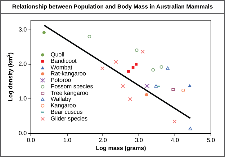
As this graph shows, population density typically decreases with increasing body size. Why do you think this is the case?

Population Research Methods

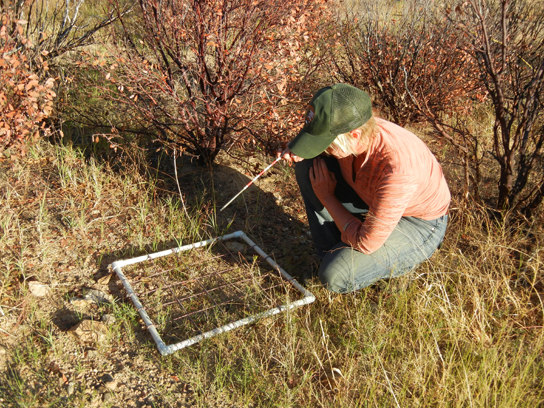
The most accurate way to determine population size is to simply count all of the individuals within the habitat. However, this method is often not logistically or economically feasible, especially when studying large habitats. Thus, scientists usually study populations by sampling a representative portion of each habitat and using this data to make inferences about the habitat as a whole. A variety of methods can be used to sample populations to determine their size and density. For immobile organisms such as plants, or for very small and slow-moving organisms, a quadrat may be used (Figure \(\PageIndex{2}\)). A quadrat is a way of marking off square areas within a habitat, either by staking out an area with sticks and string, or by the use of a wood, plastic, or metal square placed on the ground. After setting the quadrats, researchers then count the number of individuals that lie within their boundaries. Multiple quadrat samples are performed throughout the habitat at several random locations. All of this data can then be used to estimate the population size and population density within the entire habitat. The number and size of quadrat samples depends on the type of organisms under study and other factors, including the density of the organism. For example, if sampling daffodils, a 1 m² quadrat might be used whereas with giant redwoods, which are larger and live much further apart from each other, a larger quadrat of 100 m² might be employed. This ensures that enough individuals of the species are counted to get an accurate sample that correlates with the habitat, including areas not sampled.

Figure \(\PageIndex{2}\): A scientist uses a quadrat to measure population size and density. (credit: NPS Sonoran Desert Network)

For mobile organisms, such as mammals, birds, or fish, a technique called mark and recapture is often used. This method involves marking a sample of captured animals in some way (such as tags, bands, paint, or other body markings), and then releasing them back into the environment to allow them to mix with the rest of the population; later, a new sample is collected, including some individuals that are marked (recaptures) and some individuals that are unmarked (Figure \(\PageIndex{3}\)).

Figure \(\PageIndex{3}\): Mark and recapture is used to measure the population size of mobile animals such as (a) bighorn sheep, (b) the California condor, and (c) salmon. (credit a: modification of work by Neal Herbert, NPS; credit b: modification of work by Pacific Southwest Region USFWS; credit c: modification of work by Ingrid Taylar)

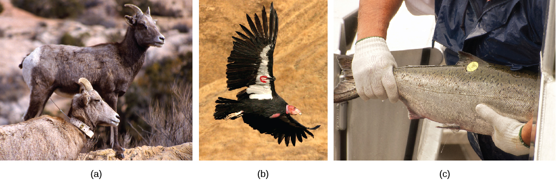
Using the ratio of marked and unmarked individuals, scientists determine how many individuals are in the sample. From this, calculations are used to estimate the total population size. This method assumes that the larger the population, the lower the percentage of tagged organisms that will be recaptured since they will have mixed with more untagged individuals. For example, if 80 deer are captured, tagged, and released into the forest, and later 100 deer are captured and 20 of them are already marked, we can determine the population size (N) using the following equation:

\[\frac{\text{number marked first catch} * \text{total number of second catch}} {\text{number marked second catch}} = N \nonumber\]

Using our example, the population size would be estimated at 400.

\[\frac{(80*100)} {20} = 400 \nonumber\]

Therefore, there are an estimated 400 total individuals in the original population.

There are some limitations to the mark and recapture method. Some animals from the first catch may learn to avoid capture in the second round, thus inflating population estimates. Alternatively, animals may preferentially be retrapped (especially if a food reward is offered), resulting in an underestimate of population size. Also, some species may be harmed by the marking technique, reducing their survival. A variety of other techniques have been developed, including the electronic tracking of animals tagged with radio transmitters and the use of data from commercial fishing and trapping operations to estimate the size and health of populations and communities.

Species Distribution

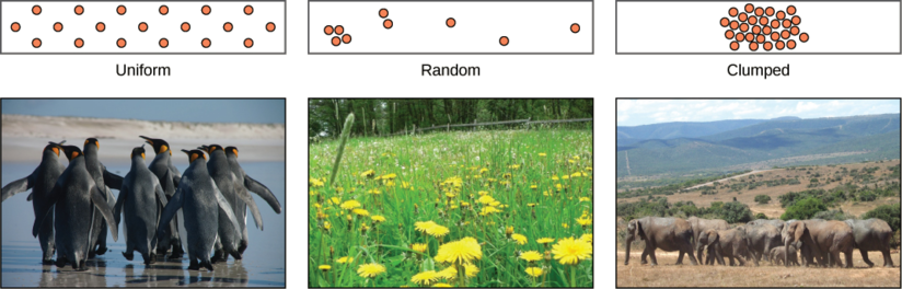
In addition to measuring simple density, further information about a population can be obtained by looking at the distribution of the individuals. Species dispersion patterns (or distribution patterns) show the spatial relationship between members of a population within a habitat at a particular point in time. In other words, they show whether members of the species live close together or far apart, and what patterns are evident when they are spaced apart.

Individuals in a population can be more or less equally spaced apart, dispersed randomly with no predictable pattern, or clustered in groups. These are known as uniform, random, and clumped dispersion patterns, respectively (Figure \(\PageIndex{4}\)). Uniform dispersion is observed in plants that secrete substances inhibiting the growth of nearby individuals (such as the release of toxic chemicals by the sage plant Salvia leucophylla, a phenomenon called allelopathy) and in animals like the penguin that maintain a defined territory. An example of random dispersion occurs with dandelion and other plants that have wind-dispersed seeds that germinate wherever they happen to fall in a favorable environment. A clumped dispersion may be seen in plants that drop their seeds straight to the ground, such as oak trees, or animals that live in groups (schools of fish or herds of elephants). Clumped dispersions may also be a function of habitat heterogeneity. Thus, the dispersion of the individuals within a population provides more information about how they interact with each other than does a simple density measurement. Just as lower density species might have more difficulty finding a mate, solitary species with a random distribution might have a similar difficulty when compared to social species clumped together in groups.

Figure \(\PageIndex{4}\): Species may have uniform, random, or clumped distribution. Territorial birds such as penguins tend to have uniform distribution. Plants such as dandelions with wind-dispersed seeds tend to be randomly distributed. Animals such as elephants that travel in groups exhibit clumped distribution. (credit a: modification of work by Ben Tubby; credit b: modification of work by Rosendahl; credit c: modification of work by Rebecca Wood)

Demography

While population size and density describe a population at one particular point in time, scientists must use demography to study the dynamics of a population. Demography is the statistical study of population changes over time: birth rates, death rates, and life expectancies. Each of these measures, especially birth rates, may be affected by the population characteristics described above. For example, a large population size results in a higher birth rate because more potentially reproductive individuals are present. In contrast, a large population size can also result in a higher death rate because of competition, disease, and the accumulation of waste. Similarly, a higher population density or a clumped dispersion pattern results in more potential reproductive encounters between individuals, which can increase birth rate. Lastly, a female-biased sex ratio (the ratio of males to females) or age structure (the proportion of population members at specific age ranges) composed of many individuals of reproductive age can increase birth rates.

In addition, the demographic characteristics of a population can influence how the population grows or declines over time. If birth and death rates are equal, the population remains stable. However, the population size will increase if birth rates exceed death rates; the population will decrease if birth rates are less than death rates. Life expectancy is another important factor; the length of time individuals remain in the population impacts local resources, reproduction, and the overall health of the population. These demographic characteristics are often displayed in the form of a life table.

Life Tables

Life tables provide important information about the life history of an organism. Life tables divide the population into age groups and often sexes, and show how long a member of that group is likely to live. They are modeled after actuarial tables used by the insurance industry for estimating human life expectancy. Life tables may include the probability of individuals dying before their next birthday (i.e., their mortality rate), the percentage of surviving individuals dying at a particular age interval, and their life expectancy at each interval. An example of a life table is shown in Table \(\PageIndex{1}\) from a study of Dall mountain sheep, a species native to northwestern North America. Notice that the population is divided into age intervals (column A). The mortality rate (per 1000), shown in column D, is based on the number of individuals dying during the age interval (column B) divided by the number of individuals surviving at the beginning of the interval (Column C), multiplied by 1000.

\[\text{mortality rate} = \frac{\text{number of individuals dying}} {\text{number of individuals surviving}} * 1000 \nonumber\]

For example, between ages three and four, 12 individuals die out of the 776 that were remaining from the original 1000 sheep. This number is then multiplied by 1000 to get the mortality rate per thousand.

\[\text{mortality rate} = \frac{12} {776} * 1000 \approx 15.5 \nonumber\]

As can be seen from the mortality rate data (column D), a high death rate occurred when the sheep were between 6 and 12 months old, and then increased even more from 8 to 12 years old, after which there were few survivors. The data indicate that if a sheep in this population were to survive to age one, it could be expected to live another 7.7 years on average, as shown by the life expectancy numbers in column E.

Table \(\PageIndex{1}\): Life Table of Dall Mountain Sheep¹

Age interval (years)	Number dying in age interval out of 1000 born	Number surviving at beginning of age interval out of 1000 born	Mortality rate per 1000 alive at beginning of age interval	Life expectancy or mean lifetime remaining to those attaining age interval
0-0.5	54	1000	54.0	7.06
0.5-1	145	946	153.3	--
1-2	12	801	15.0	7.7
2-3	13	789	16.5	6.8
3-4	12	776	15.5	5.9
4-5	30	764	39.3	5.0
5-6	46	734	62.7	4.2
6-7	48	688	69.8	3.4
7-8	69	640	107.8	2.6
8-9	132	571	231.2	1.9
9-10	187	439	426.0	1.3
10-11	156	252	619.0	0.9
11-12	90	96	937.5	0.6
12-13	3	6	500.0	1.2
13-14	3	3	1000	0.7

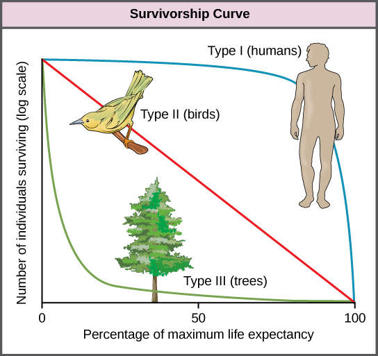
Survivorship Curves

Another tool used by population ecologists is a survivorship curve, which is a graph of the number of individuals surviving at each age interval plotted versus time (usually with data compiled from a life table). These curves allow us to compare the life histories of different populations (Figure \(\PageIndex{5}\)). Humans and most primates exhibit a Type I survivorship curve because a high percentage of offspring survive their early and middle years—death occurs predominantly in older individuals. These types of species usually have small numbers of offspring at one time, and they give a high amount of parental care to them to ensure their survival. Birds are an example of an intermediate or Type II survivorship curve because birds die more or less equally at each age interval. These organisms also may have relatively few offspring and provide significant parental care. Trees, marine invertebrates, and most fishes exhibit a Type III survivorship curve because very few of these organisms survive their younger years; however, those that make it to an old age are more likely to survive for a relatively long period of time. Organisms in this category usually have a very large number of offspring, but once they are born, little parental care is provided. Thus these offspring are “on their own” and vulnerable to predation, but their sheer numbers assure the survival of enough individuals to perpetuate the species.

Figure \(\PageIndex{5}\): Survivorship curves show the distribution of individuals in a population according to age. Humans and most mammals have a Type I survivorship curve because death primarily occurs in the older years. Birds have a Type II survivorship curve, as death at any age is equally probable. Trees have a Type III survivorship curve because very few survive the younger years, but after a certain age, individuals are much more likely to survive.

Art Connections

Figure \(\PageIndex{1}\): As this graph shows, population density typically decreases with increasing body size. Why do you think this is the case?

Answer

Smaller animals require less food and other resources, so the environment can support more of them.

Life History Patterns and Energy Budgets

Energy is required by all living organisms for their growth, maintenance, and reproduction; at the same time, energy is often a major limiting factor in determining an organism’s survival. Plants, for example, acquire energy from the sun via photosynthesis, but must expend this energy to grow, maintain health, and produce energy-rich seeds to produce the next generation. Animals have the additional burden of using some of their energy reserves to acquire food. Furthermore, some animals must expend energy caring for their offspring. Thus, all species have an energy budget: they must balance energy intake with their use of energy for metabolism, reproduction, parental care, and energy storage (such as bears building up body fat for winter hibernation).

Parental Care and Fecundity

Fecundity is the potential reproductive capacity of an individual within a population. In other words, fecundity describes how many offspring could ideally be produced if an individual has as many offspring as possible, repeating the reproductive cycle as soon as possible after the birth of the offspring. In animals, fecundity is inversely related to the amount of parental care given to an individual offspring. Species, such as many marine invertebrates, that produce many offspring usually provide little if any care for the offspring (they would not have the energy or the ability to do so anyway). Most of their energy budget is used to produce many tiny offspring. Animals with this strategy are often self-sufficient at a very early age. This is because of the energy tradeoff these organisms have made to maximize their evolutionary fitness. Because their energy is used for producing offspring instead of parental care, it makes sense that these offspring have some ability to be able to move within their environment and find food and perhaps shelter. Even with these abilities, their small size makes them extremely vulnerable to predation, so the production of many offspring allows enough of them to survive to maintain the species.

Animal species that have few offspring during a reproductive event usually give extensive parental care, devoting much of their energy budget to these activities, sometimes at the expense of their own health. This is the case with many mammals, such as humans, kangaroos, and pandas. The offspring of these species are relatively helpless at birth and need to develop before they achieve self-sufficiency.

Plants with low fecundity produce few energy-rich seeds (such as coconuts and chestnuts) with each having a good chance to germinate into a new organism; plants with high fecundity usually have many small, energy-poor seeds (like orchids) that have a relatively poor chance of surviving. Although it may seem that coconuts and chestnuts have a better chance of surviving, the energy tradeoff of the orchid is also very effective. It is a matter of where the energy is used, for large numbers of seeds or for fewer seeds with more energy.

Early versus Late Reproduction

The timing of reproduction in a life history also affects species survival. Organisms that reproduce at an early age have a greater chance of producing offspring, but this is usually at the expense of their growth and the maintenance of their health. Conversely, organisms that start reproducing later in life often have greater fecundity or are better able to provide parental care, but they risk that they will not survive to reproductive age. Examples of this can be seen in fishes. Small fish like guppies use their energy to reproduce rapidly, but never attain the size that would give them defense against some predators. Larger fish, like the bluegill or shark, use their energy to attain a large size, but do so with the risk that they will die before they can reproduce or at least reproduce to their maximum. These different energy strategies and tradeoffs are key to understanding the evolution of each species as it maximizes its fitness and fills its niche. In terms of energy budgeting, some species “blow it all” and use up most of their energy reserves to reproduce early before they die. Other species delay having reproduction to become stronger, more experienced individuals and to make sure that they are strong enough to provide parental care if necessary.

Single versus Multiple Reproductive Events

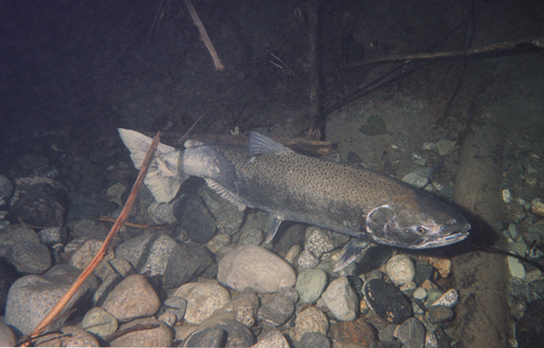
Some life history traits, such as fecundity, timing of reproduction, and parental care, can be grouped together into general strategies that are used by multiple species. Semelparity occurs when a species reproduces only once during its lifetime and then dies. Such species use most of their resource budget during a single reproductive event, sacrificing their health to the point that they do not survive. Examples of semelparity are bamboo, which flowers once and then dies, and the Chinook salmon (Figure \(\PageIndex{5}\)a), which uses most of its energy reserves to migrate from the ocean to its freshwater nesting area, where it reproduces and then dies. Scientists have posited alternate explanations for the evolutionary advantage of the Chinook’s post-reproduction death: a programmed suicide caused by a massive release of corticosteroid hormones, presumably so the parents can become food for the offspring, or simple exhaustion caused by the energy demands of reproduction; these are still being debated.

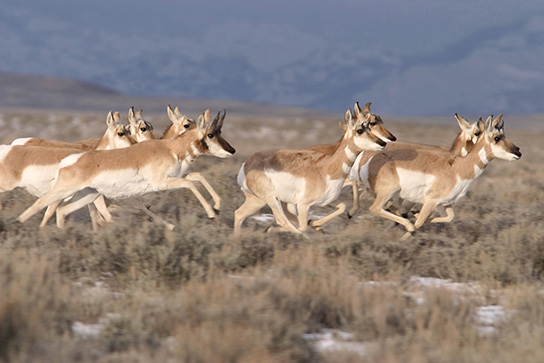
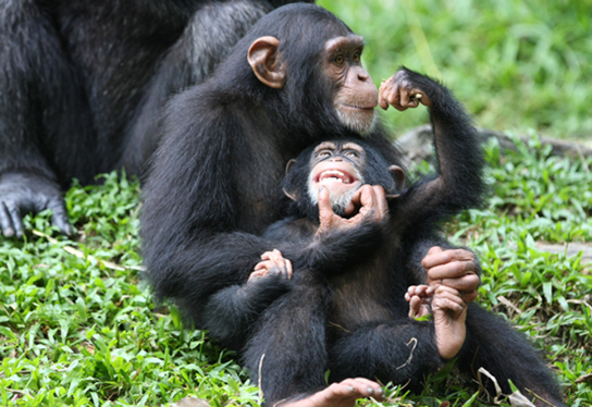
Iteroparity describes species that reproduce repeatedly during their lives. Some animals are able to mate only once per year, but survive multiple mating seasons. The pronghorn antelope is an example of an animal that goes into a seasonal estrus cycle (“heat”): a hormonally induced physiological condition preparing the body for successful mating (Figure \(\PageIndex{5}\)b). Females of these species mate only during the estrus phase of the cycle. A different pattern is observed in primates, including humans and chimpanzees, which may attempt reproduction at any time during their reproductive years, even though their menstrual cycles make pregnancy likely only a few days per month during ovulation (Figure \(\PageIndex{5}\)c).

a

b

c

Figure \(\PageIndex{1}\): The (a) Chinook salmon mates once and dies. The (b) pronghorn antelope mates during specific times of the year during its reproductive life. Primates, such as humans and (c) chimpanzees, may mate on any day, independent of ovulation. (credit a: modification of work by Roger Tabor, USFWS; credit b: modification of work by Mark Gocke, USDA; credit c: modification of work by “Shiny Things”/Flickr)

Evolution Connection: Energy Budgets, Reproductive Costs, and Sexual Selection in Drosophila

Research into how animals allocate their energy resources for growth, maintenance, and reproduction has used a variety of experimental animal models. Some of this work has been done using the common fruit fly, Drosophila melanogaster. Studies have shown that not only does reproduction have a cost as far as how long male fruit flies live, but also fruit flies that have already mated several times have limited sperm remaining for reproduction. Fruit flies maximize their last chances at reproduction by selecting optimal mates.

In a 1981 study, male fruit flies were placed in enclosures with either virgin or inseminated females. The males that mated with virgin females had shorter life spans than those in contact with the same number of inseminated females with which they were unable to mate. This effect occurred regardless of how large (indicative of their age) the males were. Thus, males that did not mate lived longer, allowing them more opportunities to find mates in the future.

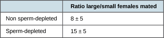
More recent studies, performed in 2006, show how males select the female with which they will mate and how this is affected by previous matings (Figure \(\PageIndex{2}\)).¹ Males were allowed to select between smaller and larger females. Findings showed that larger females had greater fecundity, producing twice as many offspring per mating as the smaller females did. Males that had previously mated, and thus had lower supplies of sperm, were termed “resource-depleted,” while males that had not mated were termed “non-resource-depleted.” The study showed that although non-resource-depleted males preferentially mated with larger females, this selection of partners was more pronounced in the resource-depleted males. Thus, males with depleted sperm supplies, which were limited in the number of times that they could mate before they replenished their sperm supply, selected larger, more fecund females, thus maximizing their chances for offspring. This study was one of the first to show that the physiological state of the male affected its mating behavior in a way that clearly maximizes its use of limited reproductive resources.

Figure \(\PageIndex{2}\): Male fruit flies that had previously mated (sperm-depleted) picked larger, more fecund females more often than those that had not mated (non-sperm-depleted). This change in behavior causes an increase in the efficiency of a limited reproductive resource: sperm.

These studies demonstrate two ways in which the energy budget is a factor in reproduction. First, energy expended on mating may reduce an animal’s lifespan, but by this time they have already reproduced, so in the context of natural selection this early death is not of much evolutionary importance. Second, when resources such as sperm (and the energy needed to replenish it) are low, an organism’s behavior can change to give them the best chance of passing their genes on to the next generation. These changes in behavior, so important to evolution, are studied in a discipline known as behavioral biology, or ethology, at the interface between population biology and psychology.

Footnotes

1. 1 Data Adapted from Edward S. Deevey, Jr., “Life Tables for Natural Populations of Animals,” The Quarterly Review of Biology 22, no. 4 (December 1947): 283-314.
2. 1 Adapted from Phillip G. Byrne and William R. Rice, “Evidence for adaptive male mate choice in the fruit fly Drosophila melanogaster,” Proc Biol Sci. 273, no. 1589 (2006): 917-922, doi: 10.1098/rspb.2005.3372.

Contributors and Attributions

Modified by Kyle Whittinghill from the following sources

• Population Demography and Life Histories and Natural Selection by OpenStax, is licensed CC BY by

  Connie Rye (East Mississippi Community College), Robert Wise (University of Wisconsin, Oshkosh), Vladimir Jurukovski (Suffolk County Community College), Jean DeSaix (University of North Carolina at Chapel Hill), Jung Choi (Georgia Institute of Technology), Yael Avissar (Rhode Island College) among other contributing authors. Original content by OpenStax (CC BY 4.0; Download for free at http://cnx.org/contents/185cbf87-c72...f21b5eabd@9.87).

• Population Dynamics and Regulation from General Biology by OpenStax (CC-BY)
• Population Demographics and Dynamics from Environmental Biology by Matthew R. Fisher (CC-BY)
• Principles of Population Growth from Biology by John W. Kimball (CC-BY)