1.11: Inheritance and Human Genetics

Patterns of Inheritance and Human Genetics

Section Overview

• Introduction: Mendel the father of modern Genetics
• Punnett squares and how to use them
• Laws of Inheritance
• Human Genetics
• Pedigrees

Pre-Lab Introduction

At this point in the semester, we have learned about DNA and how cells replicate. Now, we are going to take a step back and look at another angle -- how we get the traits we see in ourselves and each other. Our traits are determined (at least in part) by our genes. Genes are segments of DNA that encode instructions. As we learned in Lab 7, these instructions tell the cell how to make a protein. These proteins then contribute to how we look, behave, and function. We also learned about our chromosomes in lecture and in Lab 8 and that we have two of each chromosome, meaning we have two copies of every gene.

So, for every gene we have two copies. These copies are called alleles, and they don’t have to be identical to each other. Alleles code for the same type of trait but they don’t need to code for the same version. So for example, two alleles can both be responsible for eye color, but one allele codes for brown eyes while the other allele codes for blue.

Not all alleles are created equal, in that some alleles are able to dominate over others. These more prominent alleles are called dominant and are written using capital letters while the masked alleles are called recessive and shown using lower case letters. There are also alleles that create a blended appearance (incomplete dominance) as well as others that both show equally (codominance.)

Mendel the Father of modern Genetics

Johann Gregor Mendel (1822–1884) (Figure 1) was a lifelong learner, teacher, scientist, and man of faith. As a young adult, he joined the Augustinian Abbey of St. Thomas in Brno in what is now the Czech Republic.

Supported by the monastery, he taught physics, botany, and natural science courses at the secondary and university levels. In 1856, he began a decade-long research pursuit involving inheritance patterns in honeybees and plants, ultimately settling on pea plants as his primary model system (a system with convenient characteristics that is used to study a specific biological phenomenon to gain understanding to be applied to other systems). In 1865, Mendel presented the results of his experiments with nearly 30,000 pea plants to the local natural history society. He demonstrated that traits are transmitted faithfully from parents to offspring in specific patterns. In 1866, he published his work, Experiments in Plant Hybridization, in the proceedings of the Natural History Society of Brünn.

Figure \(\PageIndex{1}\): Johann Gregor Mendel set the framework for the study of genetics.

Mendel’s Experiments

Mendel’s seminal work was accomplished using the garden pea, Pisum sativum, to study inheritance. This species naturally self-fertilizes, meaning that pollen encounters ova within the same flower. The flower petals remain sealed tightly until pollination is completed to prevent the pollination of other plants. The result is highly inbred, or “true-breeding,” pea plants. These are plants that always produce offspring that look like the parent. By experimenting with true-breeding pea plants, Mendel avoided the appearance of unexpected traits in offspring that might occur if the plants were not true breeding. The garden pea also grows to maturity within one season, meaning that several generations could be evaluated over a relatively short time. Finally, large quantities of garden peas could be cultivated simultaneously, allowing Mendel to conclude that his results did not come about simply by chance.

Mendel performed hybridizations, which involve mating two true-breeding individuals that have different traits. In the pea, which is naturally self-pollinating, this is done by manually transferring pollen from the anther of a mature pea plant of one variety to the stigma of a separate mature pea plant of the second variety.

Plants used in first-generation crosses were called P, or parental generation, plants (Figure 2 ). Mendel collected the seeds produced by the P plants that resulted from each cross and grew them the following season. These offspring were called the F1 generation. Once Mendel examined the characteristics in the F1 generation of plants, he allowed them to self-fertilize naturally. He then collected and grew the seeds from the F1 plants to produce the F2 generation. Mendel’s experiments extended beyond the F2 generation to the F3 generation, F4 generation, and so on, but it was the ratio of characteristics in the P, F1 , and F2 generations that were the most intriguing and became the basis of Mendel’s postulates.

Figure \(\PageIndex{2}\): Mendel’s process for performing crosses included examining flower color. (This figure from “BIOL 310: General Biology” by Eric Wada for Folsom Lake College, “Chapter 6: Genetics” is shared under CC BY 4.0 License and was authored, remixed, and/or curated by Openstax.)

The P generation refers to?

_____________________________________________________________________________________________________________________________________

_____________________________________________________________________________________________________________________________________

What made Mendel’s Peas good subjects for studying patterns of inheritance?

_____________________________________________________________________________________________________________________________________

_____________________________________________________________________________________________________________________________________

Mendel looked at several traits of these pea plants including Stem height, Flower position, Flower color, Seed color, Seed shape, Pod shape, and Pod color (Figure 3). After breeding thousands of pea plants, Mendel noticed consistent ratios of traits would appear in the subsequent generations. These specific and predictable ratios led him to come up with several Law of Inheritance. We still use these laws today in modern genetics.

Figure \(\PageIndex{3}\): Mendel identified seven pea plant characteristics. Including seed shape and color, pod shape and color, flower color, flower positon, and stem height. (This figure from “BIOL 310: General Biology” by Eric Wada for Folsom Lake College, “Chapter 6: Genetics” is shared under CC BY 4.0 License and was authored, remixed, and/ or curated by Openstax.)

Genetic Terms used to communicate between Scientists

• Gene: The unit of hereditary, represents a portion of DNA that codes for a trait.
• Allele: An alternate form of a trait.
• Dominant allele: Requires only one copy to be expressed, regardless of what the second allele is.
• Recessive allele: Only expressed in the absence of a Dominant allele.
• Homozygous: Has two copies of the same allele.
  • Homozygous dominant: Two copies of the dominant allele.
  • Homozygous recessive: Two copies of the recessive allele.
• Heterozygous: Has two different alleles.
• Genotype: The allelic makeup of an individual for a particular gene.
• Phenotype: The expressed trait of a gene, can be observed.

Punnett Squares

Punnett squares can be used to determine the possible genotypic makeup of offspring for a given parental cross. It is important to note the results of a Punnett square are only the what is possible, the actual ratio of offspring traits may differ in some way. Why do you think this is?

_____________________________________________________________________________________________________________________________________

_____________________________________________________________________________________________________________________________________

_____________________________________________________________________________________________________________________________________

_____________________________________________________________________________________________________________________________________

_____________________________________________________________________________________________________________________________________

Now that we understand the relationship between genotype and phenotype, let’s learn how we can use this information to make predictions. We can use the genotypes of the parents to predict their offspring’s possible genotypes and phenotypes as well as their probabilities. The best way to chart these possible outcomes is to use the Punnettt square.

Figure \(\PageIndex{4}\): Giving allele designations to the various plant traits that Mendel was looking at for his experiments. R-for round seed, r- for wrinkled seed, Y- for yellow seed, y- for green seed, I- for inflated pod, i- for constricted pod, G- for green pod, g- for yellow pod, P- purple flower, p- for white flower, A- axial flower location, a- for Terminal flower location, T- for tall plant, t- for short plant. (Image taken from “Environmental Biology: an Open Educational Resource Textbook” Chapter 6 Genetics.)

1. Cross a Tall and short true-breeding pea plants using a Punnett square. Report the Phenotypic ratio.

Phenotype ratio:

_______ tall : ______ short

2. Create a cross using two of the offspring from the previous question. Report the Phenotypic ratio.

Phenotype ratio:

_______ tall : ______ short

3. Cross a Heterozygous Tall plant with a short plant. Report the Phenotypic ratio.

Phenotype ratio:

_______ tall : ______ short

Laws of Inheritance

The repeated ratios that Mendel observed in his pea plants led to his identification of laws pertaining to inheritance of traits.

Law of Dominance- Mendel recognized that one trait was dominant to its counterpart variant, suggesting there are dominant and recessive copies of traits (alleles). A dominant allele will be expressed when there is at least one copy of that allele.

Law of Segregation- The genes segregate into gametes with equal numbers of each allele or copy of a gene. This means that no one allele is more likely to show up the offspring than any other for a given cross.

Law of Independent Assortment- Genes don’t affect the inheritance of other genes in that they don’t affect the sorting of alleles into gametes. (We will talk about an exception to this law).

Review question: Remembering what we learned previously on Meiosis, how can the Law of Independent Assortment be true when the particular alleles are each on one of the paired chromosomes?

_____________________________________________________________________________________________________________________________________

_____________________________________________________________________________________________________________________________________

_____________________________________________________________________________________________________________________________________

_____________________________________________________________________________________________________________________________________

Simulating a One-Trait Cross:

Procedure:

1. Each group will pick up two paper bags filled with 15 red (R) Poker chips and 15 white (r) Poker chips. This represents two heterozygous parents (Rr x Rr). Red color being dominant to white.
2. At the same time, two students will reach into one bag and pull out one of the Poker chips. What are the only possibilities that can be made from this selection:

_____________________________________________________________________________________________________________________________________

_____________________________________________________________________________________________________________________________________

_____________________________________________________________________________________________________________________________________

3. Record your resulting genotype and phenotype in the data table for the simulated offspring from this one-trait cross of two heterozygous parents.
4. Return the Poker chips back into the bag and conduct the same process 14 more times (15 total trials).

Figure \(\PageIndex{5}\): Example of the crosses made by combing poker chips from the two parental paper bags. The colors representing the different alleles for the trait of color. White and red chip being red offspring, white and white chips white offspring, red and red chips red offspring.

Data Table 1

Trial	Offspring Genotype	Offspring Phenotype
1
2
3
4
5
6
7
8
9
10
11
12
13
14
15

Follow-up Questions

1. What is the dominant trait? __________________________________________________________________________________
2. What is the phenotype ratio of the above table? _________ Red : _________ White
3. What is the recessive trait? __________________________________________________________________________________
4. What are the genotypes of the parents? ________________________________________________________________________
5. What are the phenotypes of the parents? _______________________________________________________________________
6. Fill in the Punnett Square below using the parents given in the procedure:

Phenotype ratio:

_______ Red : ______ White

Genotype ratio:

_____ RR _____ Rr _____rr

Color of Tobacco Seedlings

Tobacco plants normally produce chlorophyll, but a mutation of a recessive allele that doesn’t code for the production of chlorophyll. The dominant allele C codes for chlorophyll and recessive allele c codes for a lack of chlorophyll. There are two possible phenotypes, producing chlorophyll (green seedlings) and non-pigmented (white seedlings).

Experimental Procedure:

1. Obtain one of the lettered images of freshly sprouted tobacco seedlings. They are all the result of a cross between heterozygous parents Cc X Cc. Using a Punnett square calculate the expected phenotypic ratio.

Phenotype ratio:

_______ tall : ______ short

2. Count the number of green and white seedlings in the image, and record the results.
   Green seedlings: _________ White Seedlings: _________
3. Reduce the counts to their most simplified ratio.
   _________ Green : _________ White
4. Did your predicted ratio match the actual observed ratio of phenotypes? _______________

Two trait crosses

It is also common to use Punnett squares to determine the probability of genotype and phenotype of two traits at once. This requires the use of a larger Punnett square 4x4 instead of a 2x2. The possible gametes also need to be determined for each parent of the cross. For this exercise we will be looking at ears of corn, that are a dihybrid cross between two heterozygous parents for kernel color and shape, P= purple p= yellow S= smooth s= rough.

When determining the possible gametes using the FOIL method is helpful, First two alleles of each trait, Outer two alleles of each trait, Inner two alleles of each trait, and Last two alleles of each trait.

Figure \(\PageIndex{7}\): Demonstrates use the foil method for determining possible gametes for a two trait cross. FOIL method is helpful, First two alleles of each trait, Outer two alleles of each trait, Inner two alleles of each trait, and Last two alleles of each trait. Gives you all the possible gamete combinations for these two traits.

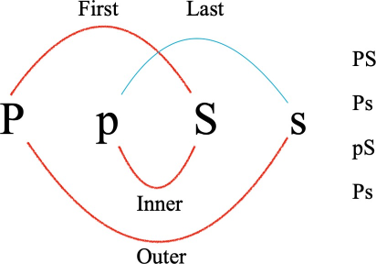
1. Determine the possible genotypes and the phenotypic ratio of a dihybrid cross. Use the foil method to determine the possible gametes.

Phenotype ratio:

_______ Purple Smooth

_______ Purple Rough

_______ Yellow Smooth

_______ Yellow Rough

2. Each lab group should get an ear of Dihybrid cross corn and count the different phenotypes present in the kernels. To avoid double counting any work in an order manner, for instance counting one row at a time. It can be helpful to work with multiple people, one counter and one recorder.
3. After you have your counts of the phenotypes present on your ear of corn fill in the below table with your results. Record your results on the board so that each lab group records one sample.

Data Table 2. Corn Dihybrid Cross Data

Sample #	Purple smooth	Purple rough	Yellow rough	Yellow rough	Phenotypic ratio
1
2
3
4
Totals

Follow-up Questions

1. In the corn experiment were the expect phenotypic ratios the same or different from the actual observed ratios?

_____________________________________________________________________________________________________________________________________

2. Was this a similar result or different from the previous exercises?

_____________________________________________________________________________________________________________________________________

3. What is the reason for the observed and expected ratios to be different?

_____________________________________________________________________________________________________________________________________

Human Genetics

Using classroom data, fill in the table below.

Trait Number of Individuals Percentage of Individuals
Hairline: Widow's Peak (WW or Ww) Straight (w)	Widow's Peak = Straight Hairline =	% with dominant trait = % with recessive trait =
Earlobes: Unattached (E) Attached (e)	Unattached = Attached =	% with dominant trait = % with recessive trait =
Tongue Rolling: Can roll tongue (R) Cannot roll tongue (r)	Can roll = Cannot roll =	% with dominant trait = % with recessive trait =
Freckles: Have freckles (F) No freckles (f)	Freckles = No freckles =	% with dominant trait = % with recessive trait =
Dimples: Present (D) Absent (d)	Present = Absent =	% with dominant trait = % with recessive trait =
Chin: Cleft chin (C) No cleft (c)	Cleft chin = No cleft =	% with dominant trait = % with recessive trait =
Pinky Finger: Bent (P) Straight (p)	Bent pinky = Straight pinky =	% with dominant trait = % with recessive trait =
Hitchhiker Thumb: Straight thumb (T) 90-degree bend in thumb (t)	Straight thumb = Hitchhiker thumb =	% with dominant trait = % with recessive trait =
Interlocking of Fingers: Left over right (L) Right over left (l)	Left over right = Right over left =	% with dominant trait = % with recessive trait =

Attribution: This section is modified from “Laboratory 9: Biology of DNA from the General Biology Laboratory Lab manual” Shared under - CC BY 4.0 License and was authored, remixed, and/or curated by Courtney Mayer (Northeast Wisconsin Technical College).

Follow-up Question

Based on the classroom data, are the dominant traits always more common?

_____________________________________________________________________________________________________________________________________

Blood Type Exercise

Blood type is based on medically relevant surface antigens found on the plasma membrane of red blood cells, and the agglutinins (antibodies) that target those specific antigens. The different surface antigens are A, B, D (also known as Rh factor), and O (a lack of A or B surface antigens). This is a case of a two trait cross represented by the phenotypes A, B, AB, O, and either positive or negative for Rh factor. We use the antibodies that target these antigens to determine a person’s blood type. This is medically relevant for blood transfusions, and can have very negative effects if a person gets the wrong type of blood. The AB blood type is a case of incomplete dominance or codominance where both the A and B surface antigens are expressed equally, and are both dominant to the type O allele.

1. For this exercise we will be looking at 4 unknown blood type samples and determining possible parentage. Using a provided blood typing kit, you will place a few drops of each sample into the three wells vertically, and then treat each well with a particular antiserum solution containing antibodies for one of three surface antigens (Figure 7).
2. Mary is Angela’s mother, your professor will provide you with their blood types. After testing the possible fathers’ blood samples fill out the below table and use what you know about genetics to determine who might by Angela’s father.

Figure \(\PageIndex{7}\): Example of the testing wells for the blood typing kit. Drops of Anti A serum in wells in row 1, drops of Anti B serum in wells in row two, and drops of Anti D serum in wells in row three. Add drops of sample 1 in wells in column one, drops of sample 2 in wells in column two, drops of sample 3 in wells in column three, and drops of sample 4 in wells in column four.

Blood Typing Results

	Mary	Angela	Sample 1	Sample 2	Sample 3	Sample 4
Blood type

3. Which sample is most likely Angela's father? ______________________________________________________________________________________________

_____________________________________________________________________________________________________________________________________

Exceptions to Independent Assortment

There are certain traits that are linked to a particular chromosome, the most common effecting humans are sex linked traits. One example being sex linked color blindness, and is a mutated allele that is only found on the X chromosome. In Humans The X and Y chromosomes determine the development of secondary sex characteristics. The X chromosome coding for the development of Female reproductive organs, while the Y chromosome codes for the development of Male reproductive organs. The typical phenotypes being XX - Female and XY - Male. In females it requires two copies of the color blind allele for them to express color blindness, but in males only having one X chromosome only need one copy of the color blind allele to express color blindness. Even though this a two trait cross, we can still use a 2x2 Punnett square to calculate the probabilities of color blindness in the offspring due to the linked nature of the secondary trait.

1. A normal vision female who’s father was color blind decides to have kids with a normal vision male, and want to know what are the chances their kids may have color blindness. Use a Punnett square to determine the female’s genotype to then do a second Punnett square cross to determine their chances of having a color blind child.
2. Report your findings for the chances of male offspring being color blind and chances of female offspring being color blind.

Genotype of Female:

_________________

Chances of Female offspring being color blind:

_________________

Chances of Male offspring being color blind:

_________________

Pedigrees for tracking autosomal disorders

Pedigrees can be used to trace patterns of inheritance by looking at several generations of a family. They can be used to trace genetic diseases while giving family history and helping provide insight for future generations.

Many conditions are genetic but the pattern of inheritance may be different depending on which chromosome the gene is found on and whether or not the mutated allele is dominant or recessive. When a mutated allele is found on the autosomes, the condition affects males and females equally. But when the mutated allele is found on a sex chromosome (X or Y), then the condition tends to predominantly affect one sex (usually male).

Figure \(\PageIndex{8}\): Example pedigree showing that there are several affected individuals, as noted by the colored-in shapes. By analyzing the relationships and connections of affected individuals, we can determine if the pattern of inheritance is autosomal dominant, autosomal recessive, sex-linked dominant, or sex-linked recessive. In this particular example, the pattern of inheritance is autosomal recessive since males and females are equally affected and the affected male on the left has two healthy parents (the “skipped generation”.) ("Pedigrees Explained" by Karen Marks, Reedley College is licensed under CC BY 4.0)

The following pedigree traces sickle cell disease through three generations of a family. Use the pedigree to answer the following questions:

Figure \(\PageIndex{9}\): Example pedigree tracing sickle cell disease through three generations of a family.

1. What is the genotype of the father in the first generation?
2. What is the genotype of the daughter in the second generation?
3. What is the genotype of individual 3 in the second generation? How do you know?
4. If the couple in the second generation has another child, what are the chances the child will have the following:
   1. Sickle cell disease
   2. Sickle cell trait
   3. Normal hemoglobin
5. If the entire family moves to an area where malaria is endemic, four of the five males in the pedigree will have a genetic advantage over the other individuals in the family. Explain why this is.

_____________________________________________________________________________________________________________________________________

_____________________________________________________________________________________________________________________________________

_____________________________________________________________________________________________________________________________________

_____________________________________________________________________________________________________________________________________

Licensing and Attributions

This Lab titled “Patterns of Inheritance and Human Genetics” is shared under CC BY-NC-SA 4.0 License and was authored, remixed, and/or curated by Tyler Wilson (Oxnard College)

Citations

• “BIOL 310: General Biology” by Eric Wada for Folsom Lake College, “Chapter 6: Genetics” is shared under CC BY 4.0 License and was authored, remixed, and/or curated by Openstax.
• “Fundamentals of Biology Lab Manual, 9: The Traits we have- Genetics and Patterns of Inheritance” shared under CC BY-NC-SA 4.0 License and was authored, remixed, and/or curated by Karen Marks and Valeria Hochman Adler for College Coalinga
• “General Biology Laboratory Manual, Laboratory 7: Meiosis and Heredity” shared under CC BY-NC-SA 4.0 License and was authored, remixed, and/or curated by Courtney Mayer (Northeast Wisconsin Technical College).
• “General Biology Laboratory Manual, Laboratory 8: Genetics of Sickle Cell Anemia” shared under CC BY 40. License and was authored, remixed, and/or curated by Courtney Mayer (Northeast Wisconsin Technical College).