1.3: Genome Assembly

Our DNA sequences are in short fragments. We need to put them together! This process is called genome assembly. The key concept for this process is "find the overlaps". If you have two reads that share a sequence, and one read ends with that sequence and the other read begins with that sequence, then you have found a pair of overlapping reads and you can basically assume that they can be combined into one. Let's look at a diagram to see why:

In this example, we have sequenced a piece of DNA and made 5 reads. If we (somewhat arbitrarily) set a rule such that we can combine reads that overlap by at least three bases, we have two sets of overlapping reads. When we squash these reads together, we create something called a "contig" (which comes from the same root as "contiguous"). In this case, were were unable to fully assemble the whole sequence because we didn't have enough reads that overlapped with each other and covered the whole sequence, so we are left with two contigs. (This is very common; it is in general very difficult to assemble a whole genome from short reads).

Now, I made that example up and found overlaps by hand. This is not how we do genome assembly! We use networks (or "graphs") to find overlaps between reads, and then we find the most efficient way to combine those reads based on overlaps. Let's start with the "overlap graph", a graph that shows which reads overlap with other reads.

Easing into it with the overlap graph

Let's say we have the following reads:

CTTAGA CCTTAG
CAGTGT AGACAG
CCCTTA
CCCCGA
TTAGAC
GACCCT
GACAGT
CGACCC

Let's construct a graph that connects any reads that overlap in at least 3 bases:

So. That actually worked, because we had enough reads and enough overlap. But! I also did that by eyeballing and by hand, and we need a more rigorous way to do that for more difficult situations.

Exercise \(\PageIndex{1}\)

Construct an overlap graph with minimum 3 overlaps to try to assemble the following reads:

AGCTAG, CACAGCT, ACGCAT, TAGCAT, ATCGAC, CACGCA, GCTAGC

Answer

CACAGCTAGCTAGCAT CACGCAT ATCGAC (you don't have enough reads to coverthe whole sequence, so you end up with 3 contigs).

The De Bruijn Graph

In many situations, we use a more complicated technique using a mathematical object called a De Bruijn graph. I'll walk you through the whole procedure here.

The first thing to do is: instead of using reads, break down each read into k-mers (aka sequences of length k). This way, we can look for overlaps in the middle of reads as well as at the end, account for potential sequencing errors, and not worry about read length. The downside of this is that we lose information about connections that are larger than the k-mers (aka we have to "reconstruct" the read as well as aseemble the rest of the genome). There are pros and cons to using this technique instead of the overlap graph, and a lot of it depends on your read lengths, coverage, and computational resources.

Exercise \(\PageIndex{1}\)

Find all the 2-mers, 3-mers, and 4-mers for the read ATGGGCT

Answer

2-mers: AT, TG, GG (2), GC, CT

3-mers: ATG, TGG, GGG, GGC, GCT

4-mers: ATGG, TGGG, GGGC, GGCT

So. Let's say I have a set of reads, and I have acquired the following k-mers from those reads where k = 3:

ACC ATA CCC ACG TAG AGA CGA GAC GAT CCT CTA TAG GAC

We're going to do something a bit weird here. We are going to split each 3-mer into 2 2-mers. These 2-mers will be the vertices of the de Bruijn graph. Each original 3-mer will be an edge of the de Bruijn graph, representing the "connection" between the 2 2-mers. So:

ACC --> AC, CC
ATA --> AT, TA
CCC --> CC, CC
ACG --> AC, CG
TAG --> TA, AG
AGA --> AG, GA
CGA --> CG, GA
GAC --> GA, AC
GAA --> GA, AA
CCT --> CC, CT
CTA --> CT, TA
TAG --> TA, AG
AGA --> AG, GA
GAC --> GA, AC

So, for example, the 3-mer GAC "links" the 2-mers GA and AC. Using this logic, we can construct a graph. Notice how I have kept the repeated 3-mer GAC.

Let's see what this graph looks like:

It's a bit weird-looking, but that's OK. The one special property of the de Bruijn graph that we are going to use is that it is guaranteed to have a path where you can hit every single node (aka it is Hamiltonian) and edge (aka it is Eulerian) exactly once. That path should, in principle, if you have enough coverage from the reads, give you the entire sequence.

Let's see if we can find a path like that in this graph by hand. (Normally we would use a computer). Notice any nodes that have fewer inputs than outputs? AT! So we should probably start there. (We should probably also end at AA, because that has fewer outputs than inputs).

Start with AT. AT goes to TA, which goes to AG. This blocks out one arrow from TA to AG. AG goes to GA (blocking out one of those two arrows). Now we have a choice. We can either go to AC or AA. If we go to AA, that's a problem, because we can't go anywhere else and we were supposed to hit every node and edge exactly once! So we have to go to AC (blocking out one of those two arrows).

Now we have another choice! We could either go to CC or CG. Let's try CC. Now, CC has a self-loop, meaning we have to go from CC to itself once. So let's do that. Then we have to go to CT, then TA, then AG again, then GA again. Now we have another choice! We still have one arrow left to AC, or we can end it at AA. We have that arrow left, so we have to try to get it. We go to AC. We went to CC last time, so the only other option is CG, then back to GA. Now we can end at AA and relax.

Our path looks like: AT -> TA -> AG -> GA -> AC -> CC -> CC -> CT -> TA -> AG -> GA -> AC -> CG -> GA -> AA. Squashing this path into a sequence yields: ATAGACCCTAGACGAA.

Exercise \(\PageIndex{1}\)

Try the choice when we are first at AC but decide to go to CG instead of CC. Can you make an Eulerian path? What do you notice is different?

Answer

AT->TA->AG->GA->AC->CG->GA->AC->CC->CC->CT->TA->AG->GA->AA

Yes, but it's a slightly different sequence!

ATAGACGACCCTAGAA. The "GAC" and "CCTA" blocks are switched. Either of these are possible solutions.

You will notice after doing that exercise that there are two possible solutions to this assembly. How can we figure out which one is correct? Well, we usually would try a bigger size of k. Here is the corresponding list of 4-mers, and the corresponding de Bruijn graph.

TAGA CGAT ATAG ACCC GACC AGAC TAGA CCTA CCCT CTAG GACG AGAC ACGA

TAGA --> TAG, AGA
CGAT --> CGA, GAA
ATAG --> ATA, TAG
ACCC --> ACC, CCC
GACC --> GAC, ACC
AGAC --> AGA, GAC
TAGA --> TAG, AGA
CCTA --> CCT, CTA
CCCT --> CCC, CCT
CTAG --> CTA, TAG
GACG --> GAC, ACG
AGAC --> AGA, GAC
ACGA --> ACG, CGA

Now this one is much easier to deal with. You can basically read off the only possible Eulerian path: ATA -> TAG -> AGA -> GAC -> ACC -> CCC -> CCT -> CTA -> TAG -> AGA -> GAC -> ACG -> CGA -> GAA. So our sequence is ATAGACCCTAGACGAA (aka the first choice in the 3-mer version).

Why would anyone choose a smaller value of k? Well, it is important to remember that a lot of the limitations of bioinformatics problems are computational; sometimes we don't have the resources to do massive computations so we have to make do with smaller ones and hope for the best.

Once you have created contigs from reads by some sort of graph-based method like these, you can partially link these contigs together into scaffolds, which are basically contigs connected by a known sequence length but an unknown sequence. This is performed using molecular biology techniques and physical evidence, and has the benefit of adding more structure to your assembly even if you don't know exactly what sequence is connecting the contigs. Assembly programs can attempt to fill in these gaps and figure out the sequences, especially in the case of assembling against a reference. Note that contigs from different chromosomes should never be connected!

How do you evaluate a de-novo assembly?

A de-novo assembly is what we have been doing so far, trying to put together a genome from scratch, from just the reads. If you had a reference genome, you could use that reference genome to help you assemble your genome, and the problem becomes much easier. BUt we'll focus on de-novo assembly for this chapter. So, how do you know you did a good job on the assembly?

There are a few different ways to evaluate an assembly, and I'll go through each of them here.

Contig Length Distribution

The number one thing you want out of an assembly is to put as many reads together on a single contiguous segment of DNA as possible. Ideally, we would want one single contig consisting of all the reads, but that is usually impossible unless you have very long reads and/or a very short genome. So, we evaluate our assembly by how well it achieved the target of

1. small number of contigs that are
2. very long and
3. contain as many of the reads as possible

There are a few ways to measure this, and they are all measured by a program called QUAST, so I will use that program as an example here.

The most basic measurements are: total # of contigs, the length of the longest contig, the total number of bases in all the contigs, and the total number of bases in the reference genome (if there is a reference). You can also report GC content of the assembly and the reference to see if something weird happened (i.e. you want the GC contents to match). These numbers are mildly useful (you generally want a small # of contigs, a large length of the longest contig, and the total number of bases in all the contigs to be as close as possible to the total number of bases in the reference genome), but consider the following scenarios:

1. two contigs, but almost all reads are unassembled
2. one large contig that contains 30% of the genome, and then 100,000 small contigs

Neither of these are good scenarios, and you wouldn't be able to tell just by looking at the total # of contigs (in the first case) or the length of the longest contig (in the second case). Along with these "absolute" measurements, we need some measurements that look at the whole distribution of contig lengths.

Let's start with an example. Consider the following two read length distributions:

Assembly 1	Cumulative	Cumulative Percentage	Assembly 2	Cumulative	Cumulative Percentage
3383	3383	33.83	1579	1579	15.79
2110	5493	54.93	1458	3037	30.37
2023	7516	75.16	1211	4248	42.48
1023	8539	85.39	1022	5270	52.70
782	9321	93.21	872	6142	61.42
345	9666	96.66	845	6987	69.87
202	9868	98.68	786	7773	77.73
76	9944	99.44	772	8545	85.45
41	9985	99.85	751	9296	92.96
15	10000	100	704	10000	100

The main two numbers we want to compute here are called N50 and L50. N stands for "number", and L stands for "length". The "50" is the key concept here; we are focused on obtaining 50% of the total genome size. (You can adjust this number to any percentage you like, depending on what standard you want, but the default is 50% People sometimes look at the entire range of possible percentages; this is a bit more of a thorough approach and I would recommend it; my online application shows all of them). The question is: what is the minimal number of contigs you need to get 50% of the assembly? (You want this number to be small; you want most of the genome to be captured by as few contigs as possible). The number that answers this question is L50. For assembly 1, L50 = 2 (you just need the two longest contigs to hit 50%). For assembly 2, L50 = 4 (you need the 4 longest contigs to hit 50%).

Another question to ask is: what is the length of the shortest contig used for 50% of the assembly? This is the length of the shortest contig used when calculating L50. As usual, you want this number to be big. For assembly 1, this length is 2110 bases, and for assembly 2, this length is 1022 bases.

One thing to note about these numbers is that they depend on the length of the assembly. So, if you want to compare across assemblies, it's better to look at 50% of the estimated genome size rather than the assembly size (total number of bases in assembly); this version of these statistic are called LG50 and NG50. In our example above, both assemblies have the same size (10,000 bases) so we can compare them directly using L50 and N50.

One infuriating thing is that these two statistics are named backwards! The "N" one measures Length, and the "L" one measures Number! The good news is that L50 is unitless and N50 is in units of bases, so as long as you are careful and report numbers in the appropriate units then it doesn't really matter if you accidentally mix them up.

Exercise \(\PageIndex{1}\)

Which assembly above, 1 or 2, would you prefer to work with? Why? (Don't just say e.g. "because N50 is bigger/smaller"; explain why having a larger or smaller value is better).

Answer

Assembly 1. N50 and L50 are both bigger. For both statistics, we want them to be as large as possible because we want as much information as possible to be on as few contigs as possible. One giant contig and a billion small contigs is probably better than ten evenly-sized contigs, because in the latter case there is no way to combine those contigs together to get the information you get from the giant contig in the first case.

Using Biological Information: BUSCO

There are genes that are highly conserved across all organisms (aka they are very similar across all organisms, usually because they are so important that any mutation would be bad). One way to see if your assembly is good is if it contains these genes, ideally in one piece. BUSCO (Benchmarking Universal Single-Copy Orthologue) is a method that checks for these genes. In particular, BUSCO looks at single-copy genes that are present in the taxonomic clade of interest (using ortholog data from here) and tries to fin them in your assembly sequence. Here is an example output from a BUSCO analysis (from the user manual):

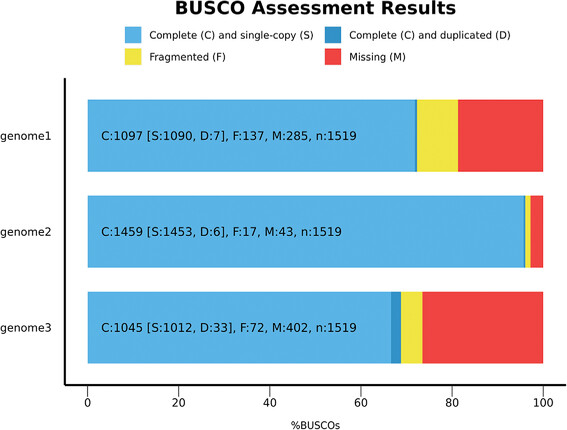
These are three example genome assemblies. The x-axis tells you how many of the BUSCO genes were missing (red), present but fragmented (yellow), present, complete, and duplicated (darker blue) and present and in a single-copy (blue). Because these genes are only ever present in a single copy, a duplication indicates an assembly error.

In general, you want as much as possible to be complete and in a single copy.

k-mer Methods

So far we have looked at the specific contig lengths and also tried to find highly conserved single-copy genes. There is a third "angle" at which we can come at assessing de-novo assembly: checking to see if the assembly itself is consistent with the reads it came from. For these methods, we pick a k, find all k-mers present in the reads, find all k-mers present in the assembly, and compare how many times each k-mer occurs in the reads vs. the assembly.

The count of a particular k-mer in the read set is somewhat irrelevant, as it depends on read depth and there could be many many reads from the same sequence. However, in the assembly, the k-mer count is important, because we are making one genome. In a diploid organism, we would expect most k-mers to appear in the assembly twice, with those appearing once indicating heterozygosity. Ideally, every read will fall into one of these categories, and anything else indicates some sort of assembly error (mapping too many different reads to the same place, perhaps). k-mers that are unique to reads (aka not in the assembly) usually only appear once and probably indicate sequencing error, and k-mers that are unique to the assembly but not in the reads indicate some sort of assembly error at the base level. Below is a plot from the software package Merqury, which performs these kinds of analyses.

On the left (a) is a histogram of the k-mers looking just at the reads from an NGS experiment. There is a peak for 2-copy k-mers (homozygous) that occur about 45 times each, 1-copy k-mers (heterozygous) that occur about 45/2 = 22.5 times each, and a peak of k-mers that only occurs about once or twice. If every "proper" k-mer occurs 22.5 times to one particular locus, then these unique k-mers are probably just sequencing errors.

On the right (b), we count how many times each k-mer comes up in the assembly. Those weird unique k-mers that are probably sequencing errors don't show up at all. The 1-copy and 2-copy kmers appear almost always in the 1-copy and 2-copy spots, so that's good. Some k-mers appear more than twice in the assembly, which indicates an assembly error of some kind, but these are rare. There are also k-mers that are only found in the assembly, which also indicates an error. In general we want almost everything to be within those two main peaks.

Lab Activity

A lab activity can be found at this GitHub link in the compressed folder "assembly_lab.zip". Inside, there is an RMarkdown file that contains instructions as well as data files.