1.2: DNA Sequencing

The basic starting point for much bioinformatic analysis is a DNA or protein sequence. In this chapter, we discuss DNA sequencing methods.

Learning Objectives

• Describe the basic methods of first-generation (Sanger), next-generation, and nanopore sequencing
• Compare and contrast the pros and cons of each sequencing method
• Evaluate which sequencing method is most appropriate for example scenarios
• Understand how to interpret raw sequencing data
• Recognize potential errors in sequencing
• Describe quality control methods for post-processing raw sequence data

First Generation Sequencing

The very first successful method of sequencing DNA was developed by Frederick Sanger and others (and is therefore called Sanger sequencing). The technique uses a very common principle in molecular biology: if we want to do something to a biological system, let's use how biology does it!

The method is based off of DNA replication, where you have the DNA strands you want to sequence, the DNA polymerase enzyme that replicates the DNA, and a large supply of nucleotides (that will make up the replicated DNA). There are two tricks, though:

1. You also need a small amount of "broken" nucleotides. These nucleotides, once added on the growing replicated DNA, have sort of a "snub end" so that other nucleotides cannot attach onto them. Thus, the replication stops after a broken nucleotide is added. Because this process is random, you get fragments of varying lengths. If you have just the right amount of these "broken" nucleotides compared to the normal nucleotides, you can get sequence fragments of every length, as there is a decent probability that some of the DNA replication has stopped at each point.
2. The other trick is that these "broken" nucleotides are labeled (originally radioactively, but now we use fluorescence) in four different "colors", so we know which nucleotide stopped the replication. Thus, we know exactly the identity of the base at that position

Once we have all of these fragments, we run them through a gel electrophoresis, which is a technique that separates molecules based on their size. In this case, the size of the DNA is the length of the DNA, so the fragments are ordered from shortest to longest. Because we know what nucleotide is at each length, we can reconstruct the full sequence of the DNA. The below figure shows this process.

Note

Another early method, developed by Allan Maxam and Walter Gilbert, was also developed around the same time as Sanger's method. This alternative method used precise chemistry to break the DNA at specific bonds between specific nucleotides (for instance, you could break the DNA every time there was a C). This method was initially more popular than Sanger sequencing because you could just use the original DNA and didn't have to create many many copies of the original DNA like you do in Sanger sequencing, but overall it is much more technically challenging and is no longer used today.

Reading Sanger Sequencing Output

These days, the output of Sanger sequencing is either an ab1 file or an scf file, which can be viewed in a variety of different software packages. We will take a look at Sanger sequencing output in the R activity.

Sanger sequencing is still commonly used today. It is best used when you are studying only a few genes and want long, accurate read lengths. Another benefit is that the technology used is relatively simple and familiar to many biologists. Once you start needing to sequence many genes, however, Sanger sequencing becomes very expensive and slow. Which brings us to the next generation of sequencing techniques!

Next-Generation Sequencing (NGS)

The most popular "next-generation" style of sequencing was pioneered by people whose company was bought by the company Illumina, hence this type of sequencing is called Illumina sequencing. This method has two basic ideas: make a very large number of small DNA fragments, each with many identical copies, and then anchor them to a surface. Next, replicate the DNA one base at a time using fluorescently tagged dNTPs, then record the fluorescence for each strand, wash away the dNTPs, and repeat. The benefit of this technique is that you make many identical copies of DNA, so the error rate is small. In addition, you can sequence many different strands of DNA at once. The downside is that the DNA fragments themselves have to be small, so putting them together into a full sequence is challenging and will be the subject of next chapter.

Another NGS method is performed by the company PacBio, hence this type of sequencing is called PacBio sequencing. The basic idea of this method is to observe the replication of the DNA directly. Each fragment of DNA is at the bottom of a small hole, and a small fluorescent detector reads each base that gets attached. The advantage of this method is that the reads are much longer, but the disadvantage is the the error rate is a bit higher than Illumina sequencing and it is also a bit more expensive.

Finally, the most modern sequencing technique is called nanopore sequencing, and has been spearheaded by Oxford Nanopore Technologies. The basic idea of this method is to push a DNA strand through a small hole, and measure changes in charge to detect each base. The advantage of this method is that it can create extremely long reads and can be portable, but the error rate is much higher. These various techniques are compared in this table (all numbers are approximate):

Method	Company	Price	Read Length Max	Pros	Cons
Sanger	Various	$5 per sequence	1kbp	Cheap, accurate	Small datasets
Next-generation sequencing	Illumina, Thermo Fisher	$200 per genome	300bp	Large datasets (up to whole genome)	More difficult to access
Long-read sequencing	Oxford Nanopore, PacBio	$1000 per genome	4Mbp	Very long reads	Expensive, slow, somewhat inaccurate

The "cons" for NGS and long-read sequencing are quickly being improved upon by continued technilogical advances.

Quality Control of Raw NGS Reads

In the sequencing of DNA fragments, each base gets a quality score provided by the sequencing machine based on a calibrated likelihood of mis-identifying a base. These quality scores are also called "Phred" scores. If p is the probability of an error, then the quality score is

\[ Q = -10 \times \log_{10}(p).\]

Thus, Q = 30 means that the probability of calling a base incorrectly is 0.001. The higher the value of Q, the better the quality of the base call. Because we want to encode this value in a single character (so that we can put the sequence and the Q score next to each other in a FASTQ file), we use ASCII characters from the following table (obtained from https://www.drive5.com/usearch/manua...ity_score.html).

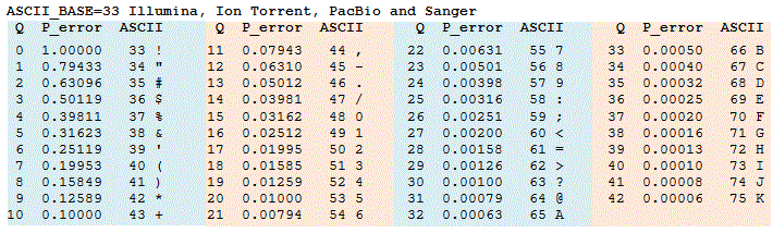
If you want to eyeball a FASTQ file for error rates, if you see a series of symbols (especially !), then your qualities are low, and you have A-K from the alphabet then the qualities are high.

What do you do with low-quality base calls? Well, if the whole thing is bad we have to re-do the experiment. However, usually we just filter out reads that are not sufficiently high-quality prior to assembly and alignment (the next two chapters).

There are other things we can look at to see if the quality of our reads is good, and most of these are general sanity checks. For example, we can take a look at the frequency of each base; these should remain consistent across all reads at each cycle (aka increase in length). We can also look at GC content, which is the fraction of bases that are G or C. This fraction is relatively consistent within species but can vary quite a bit across species; if your GC content is well outside the expected range for your species, then there might be some contamination.