1.4: Genome Alignment

Suppose you have a sequence, or at least a series of contigs. What do you do next? One thing you can do is align that sequence to a reference genome that you already know a lot about. Aligning a sequence to another one is basically just matching the two to each other. There are many reasons you would want to do this, including finding similar genes, finding homologous genes (similarity by evolutionary history), comparing genomes, and assembling reads using a reference.

We'll start by defining what a "match" is, then we'll go through three algorithms that we use to align genomes.

PAM Matrix

So what is a "match"? How different are different parts of a sequence?

If we are doing, say, a Google search, and we want an exact match, we put quotes around the query (e.g. "alignment to a reference genome" will search for this exact sentence). By contrast, if you just put that phrase in without quotes, you can get those words mostly in the same order, but possibly with other words in between. When we align genomes, we want to leave room for gaps and mutations, so the process is more similar to the second kind of search.

If we have a DNA sequence, the simplest model to use is to treat every mismatch as equal. So e.g. A vs T is the same as A vs G. However! Some mutations are more likely than others, so if you wanted to be a bit more accurate you'd treat the less likely mutations as being "further apart". We'll go over these mutation rates more in the chapter on phylogenetics.

When we align sequences, we usually want to use the protein (amino acid) sequence, as there's more information there (we can ignore silent mutations). Of course, when we build a tree and do phylogenetics, we want to use the DNA sequence because silent mutations still provide useful information about phylogeny, but here we're just trying to line up some strings. Now, amino acid changes are way more complicated than nucleotide changes. What constitutes a "similar" amino acid, or a "likely" change, or an "unlikely" change? The first attempt at creating a matrix that tells you how much to "score" a match or mismatch based on sequence similarity was performed by the founder of bioinformatics, Margaret Dayhoff (see Box BOX). This matrix was called the PAM (point-assisted mutation matrix), and was obtained by looking at different sequences of highly-conserved proteins and seeing how often various amino acid changes happen. The original PAM matrix was used for a while, but has recently been superseded by a matrix called the BLOSUM matrix, which uses sequences that slightly more diverged and can be more accurate over less closely-related sequences.

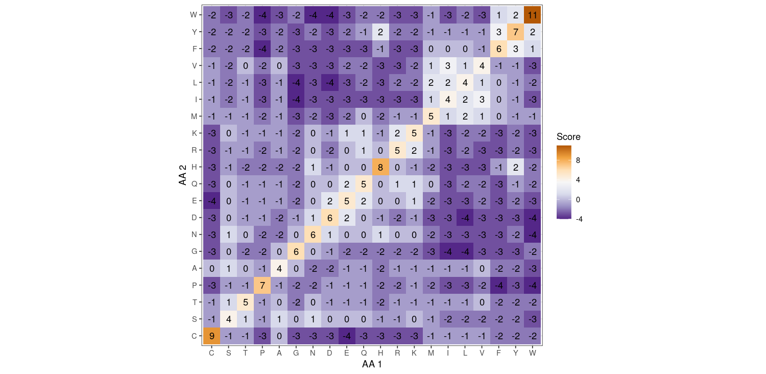
How you use this matrix is: line up your two sequences, and compare the two amino acids at each position. Add up the scores you get from each comparison. For the BLOSUM matrix, a higher score is better (aka most matching). These numbers are log-odds: you take the probability that you get a particular pair (say, T in one sequence and M in the other sequence) and divide that by the probability that you would get that pair just by randomly pairing up the two sequences (so if T and M were very frequent, you'd be likely to get that pair randomly anyways). A positive number means you are more likely to get that pair by chance, and a negative number means you are less likely to get that pair by chance.

Exercise \(\PageIndex{1}\)

1. First, let's consider the diagonal. AKA, if you see a "C" in both sequences, you add +9. If you see a "Q" in both sequences, you add +5. Which amino acid are you less likely to see pair with itself by chance? That is, between C and Q, which one tends to have more mutations away from it?
2. Name the most likely substitutions and the least likely substitutions.

Answer

1. Q; the log-odds of seeing QQ is lower than seeing CC
2. The highest positive off-diagonal value is 3, which is the I/V substitution. The lowest negative value is -4, which occurs for W/P, W/N, W/D, F/P, L/G, L/D, I/G, and E/C.

Needleman-Wunsch Algorithm

Now that we have a way of scoring an alignment to see how good it is, we need to make that alignment in the first place! As with everything else, "eyeballing" isn't good enough; we need an algorithm to use. We'll start with the Needleman-Wunsch algorithm, which is used for global alignment (aka let's align the entire sequences together with gaps if necessary; this is opposed to local alignment where we care about aligning some part of each sequence together and may not care about the whole thing).

We start with two sequences we want to align:

AGCTACAT
ACTAGCAT

In general, we would use a fancy scoring matrix like a PAM or BLOSUM matrix, but for this demonstration we'll use a simple scoring system: a match is +1, a mismatch is -1, and a gap is -2.

We start by making a big grid with one sequence on top and the other sequence on the side. We have a blank label for the first row and first column, and always start by putting a "0" in the top-left.

Now, each cell is going to be filled out by row, so you start from the top left and move left-to-right. For each cell, you take the maximum of the following three values:

1. The score above minus the gap penalty
2. The score to the left minus the gap penalty
3. The score to the diagonal top-left plus the match score if this row and column is a match or minus the mismatch penalty if this row and column is a mismatch

In an alignment with no gaps, all we are doing is comparing matches and mismatches, and we'd be going down the diagonal and using only the 3rd number. However, this algorithm allows us to incorporate gaps by shifting either up/down or left/right (for a gap) and then continuing down diagonally bottom-right as we continue matching up the alignment.

Filling out the first row this way is different from everything else because there is no "above" row so we just use calculation 2. Similarily, for the first column, there is no "left" column so we just use calculation 1. In both these cases, we just subtract the gap penalty over and over.

OK, now let's start at the next thing to be filled in, which is the top-left empty space. Calculation 1 is "-2 - 2 = -4", where the first -2 is the top score, and the second -2 is the gap penalty. Calculation 2 is also "-2 - 2 = -4", where the first -2 is the left score. Calculation 3 is "0 + 1 = 1" because it's a match (A and A). The maximum between -4, -4, and 1 is 1, so we fill that in. Notice that in our scoring system, gaps are worse than mismatches, so when we do the full alignment we may allow more mismatches than gaps. In general, you can change your scoring system to weigh gaps more or less heavily than mismatches, depending on how many gaps you might expect in your alignment.

Now we move one cell to the right. Calculation 1 is "-4 -2 = -6". Calculation 2 is "-2 -2 = -4". Calculation 3 is "-2 -1 = -3" because G and A are a mismatch. The maximum of -6, -4, and -3 is -3, so we fill in -3.

I have filled the rest of the table in.

From this table, we find the optimal alignment by starting at the bottom left and then tracing a path through this table. At each cell, find the highest number from either its top neighbor, left neighbor, or top-left diagonal neighbor, and then go there. If multiple numbers of those three are equal, those represent equally valid optimal alignments, so you have to go down those different paths separately. If you choose the diagonal, then write down both of the corresponding bases/amino acids. If you choose to go up, that means its a gap in the side sequence aligned with the letter in the top sequence, and if you choose to go left, that means its a gap in the top sequence aligned to the letter in the side sequence. So. Let's do this for our example.

The alignment that you can read off of this table (remember when you write this down you start at the end and go backwards) is:

Top: T -> AT -> CAT -> -CAT -> A-CAT -> TA-CAT -> CTA-CAT -> GCTA-CAT -> AGCTA-CAT
Side: T -> AT -> CAT -> GCAT -> AGCAT -> TAGCAT -> CTAGCAT -> -CTAGCAT -> A-CTAGCAT

Was that the alignment you would have come up with just by eyeballing? Probably. But we use this algorithm for much longer sequences where things are not as straightforward.

The Needleman-Wunsch algorithm is used for global alignment; we want to align the whole sequences together as well as possible. If we were concerned about local alignment (aka we know that most of the sequence will not align very well but we hope that some portion of it does), then the algorithm we use is a slightly modified version called the Smith-Waterman algorithm.

The main differences between the Needleman-Wunsch (NW) and Smith-Waterman (SW) algorithms are:

1. No negative numbers for SW. You can imagine that in the NW algorithm, large regions of mismatch would lead to a buildup of negative numbers that is a "hole" that partially-aligning parts of the sequence won't be able to "dig out of", and so sequences that align poorly overall are going to have horrible scores even though they align well in certain specific places. The SW algorithm makes all numbers that would be negative in NW zero, so that you can kind of "start fresh" every time there is a bad set of mismatches. The way this is implemented is that for NW, there were three numbers you had to find the maximum of, but in SW if that number ends up being negative you force it to be 0.
2. Instead of starting at the bottom-right and ending at the top-left (aka aligning the whole sequence), you start at the highest number and end once you hit 0 (aka you are trying to find the best partial (aka local) alignment between the two sequences.

Here I have performed the SW algorithm instead of the NW algorithm on this example.

Notice that there are few places we could have started if that last "T" wasn't there (one is highlighted in bright green; the other two are part of the solution), and these correspond to places where the sequences align locally but the matching parts are in different places overall (e.g. "AGC" is in both, and "CTA" is in both). But because the last "T" has that "4", we have to start there.

The optimal local alignment here is

Top: T -> AT -> CAT -> -CAT -> A-CAT -> TA-CAT -> CTA-CAT
Side: T -> AT -> CAT -> GCAT -> AGCAT -> TAGCAT -> CTAGCAT

Almost the same as the NW result, but we stopped before aligning first two bases of the top sequence or the first base of the bottom sequence. That's because our gap penalty is high compared to our mismatch penalty. A high gap penalty will lead to a lot of zeros, so you'll end up stopping instead of trying to put a gap in more frequently.

Here is the same alignment, but with the gap and match/mismatch penalties switched in magnitude (so gaps are -1, matches are +2, and mismatches are -2).

This alignment looks like:

Top: T -> AT -> CAT -> ACAT -> -ACAT -> T-ACAT -> CT-ACAT -> GCT-ACAT -> AGCT-ACAT
Side: T -> AT -> CAT -> GCAT -> AGCAT -> TAGCAT -> CTAGCAT -> -CTAGCAT -> A-CTAGCAT

So this is a different result! We managed to align the whole thing, but this time something different happened at around the 5th base. So this example demonstrates that sometimes it does matter what penalties and scores you use.

Exercise \(\PageIndex{1}\)

Use the Needleman-Wunsch Algorithm to align the following sequences:

ACGTGA

AGTGA

Using: matches = +2, mismatches = -1, and gaps = -2.

Answer

 

	-	A	G	T	G	A
-	0	-2	-4	-6	-8	-10
A	-2	2	0	-2	-4	-6
C	-4	0	1	-1	-3	-5
G	-6	-2	2	0	1	-1
T	-8	-4	0	4	2	0
G	-10	-6	-2	2	6	4
A	-12	-8	-4	0	4	8

ACGTGA

A-GTGA

Multiple Sequence Alignment

So far we have only been talking about how to align two sequences to each other (aka pairwise alignment). Frequently, however, we need to align multiple sequences together simultaneously. One use for this is in building phylogenetic trees: you need to know how different the sequences are, and for that you need to directly compare homologous sequences across multiple samples. We could align every pair of samples separately and compute some sort of genetic distance between the two samples, and use a distance-based phylogenetic method. However! There is a lot of potential information in the other samples that you could use to help align them all better with each other, doing all pairs is computationally inefficient, and there are better phylogenetic methods than distance-based ones that require the simultaneous alignment of multiple samples. So let's see how we do this.

The most common technique for doing a Multiple Sequence Alignment (MSA) is via progressive alignment. This is an iterative process that starts with unaligned sequences and creates a pairwise distance matrix between them, usually starting with a pairwise alignment method that I described above. This distance matrix is used to make a distance-based tree that is used to divide the alignment problem into smaller problems; this tree is called a "guide tree". Then, small groups of sequences that are clustered together on the guide tree are aligned separately, and once those alignments are complete, the groups are aligned with each other.

There are many different algorithms you can use for an MSA, and some of them are better in different circumstances. The most popular right now are MAFFT, MUSCLE, and ClustalOmega. Here is an example of an MSA produced by ClustalX (an older version of Clustal):

(By Miguel Andrade at English Wikipedia - Transferred from en.wikipedia to Commons., CC BY-SA 3.0, https://commons.wikimedia.org/w/inde...?curid=3930704)

Each row is a sample seuquence, and each column is a site. In this case, we are looking a protein alignment, so the sites are amino acids. A dash indicates a gap. Colors can indicate many different things in a MSA; in this case they are related to the properties of the amino acid (basically, the same color means the same amino acid, and a color is shown if the amino acid is highly conserved across sequences and share similar properties). By visualizing alignments like this, we can see how successful they are and quickly spot mutations. Amino acid properties include things like polarity/hydrophilicity.

Exercise \(\PageIndex{1}\)

In the above alignment:

1. What do you think the asterisk (*) stands for?
2. What is the most common length of this protein?
3. Between what 20bp stretch between 10bp markers is the protein most conserved? What about most variable?

Answer

1. All samples have the same amino acid
2. 76 aa
3. 60-80, 1-20

Lab Activity

A lab activity called "alignmentlab.pdf" is part of the supplemental files for this textbook. An Rmarkdown file of this lab can be found at this link.