2.13: Population Ecology

What is population ecology? 

Thousands of bird species breed and reproduce in North America.  Some, like the American Robin (Turdus migratorius), are widespread, and can be found building nests and raising their young in every state of the USA, several Canadian provinces, and many locations in Mexico.  Others, like Kirtland's Warbler (Setophaga kirtlandii) breed almost entirely within a single state (Fig. 9.1.1); a few, like the Cozumel thrasher (Toxostoma guttatum) and Socorro mockingbird (Mimus graysoni) are found only on single small islands.  Population ecologists study what determines the occurrence and abundance of species in space and time: their geographic ranges, population sizes and densities, and what factors result in them being so rare or common.  

Ecology is often defined as the study of the distribution and abundance of organisms. Population ecology is the branch of ecology that works to understand the patterns and processes of change over time or space for populations of a single species. Population ecology is the science of population dynamics in space and time.  A species is typically defined as a group of organisms capable of interbreeding. For some species, all of the members of the species occur in the same geographic area and could potentially meet and interbreed during their lifetimes. Most species, however, can be divided into geographically separate populations. Individuals within a single population are likely to interact and perhaps inter-breed, while those from different populations will only come into contact if there is long-range movement between the populations (dispersal).

Populations can be described by their size, density, or spatial extent

One species that currently consists of a single population is the Kirtland’s warbler (Setophaga kirtlandii), a North American songbird. Almost all members of this species occur in the northern part of the state of Michigan in the United States (Figure \(\PageIndex{1}\)). In contrast, the Spotted Owl (Strix occidentalis) is a species with many distinct populations throughout the western United States, southern Canada, and central Mexico.

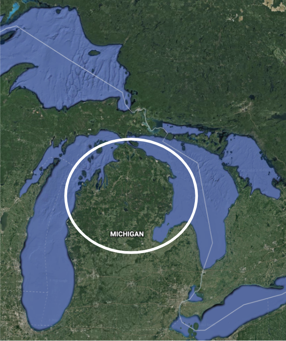
Figure \(\PageIndex{1}\): Left: "A male Kirtland's Warbler Setophaga kirtlandii in a forest in Michigan, USA" by Jeol Trick is licensed under CC BY 2.0. Right: Core habitat area of Kirtland's Warbler. Source: Google Earth: https://bit.ly/3ofgDK1. 

 

For both species and populations, patterns of distribution and abundance can be considered in several ways. These include:

1. Size: How many total individuals there are?
2. Density: How many individuals per unit of area?
3. Dispersion: How are individuals in a population arranged spatially relative to another?  Do they occur in clumps or are they evenly spread apart?
4. Occupancy: Does a species or member of a population occur in a given habitat, or is it absent?
5. Population distribution: Where does a population occur in space?
6. Geographic range: What are the furthest geographic limits of where a species occurs?

In addition to static characteristics of size and distribution, populations are dynamic and fluctuate based on a number of factors: seasonal and yearly changes in the environment, natural disasters such as forest fires and volcanic eruptions, and competition for resources between and within species. To study these many facets of a population's biology, ecologists use both systematic field observations to determine its current status, and mathematical tools to characterize how it responds to changes in the biotic and abiotic environments.

Population size is the number of individuals in a population

Population size is the actual number of organisms in a population. This is often of great interest to biologists – especially those working in forestry, wildlife management and conservation – and most of our basic population models work with population sizes. A complete census is one way to determine population size and entails counting each individual present within the population. This occurs in some well-studied populations, such as the Kasekela population of chimpanzees in Gombe National Park, Tanzania (Pusey et al. 2008), and the Seychelles Warbler on islands in the Indian Ocean off the coast of East Africa (Burt et al. 2016).

Although it is the most accurate methodology, counting every individual in a population can be difficult, if not impossible.  In most cases ecologists can only attempt to estimate the population size (N) by using well-designed field studies and statistics. Indeed, some population ecologists specialize in developing mathematical and statistical models to accurately estimate population size, such as mark-recapture models and camera-trapping methods (detailed below).  Often, however, we do not have good estimates of the size of a population itself, but factors that should be correlated with the population size, such as the number of animals harvested by hunters or trapped by ecologists or the density of dung found during a survey. 

Data that we think correlates with actual abundance constitutes a population index.  Index data are cheaper to collect than the data needed for formal estimates of population size such as the mark-recapture methods discussed below, but can be biased and provide an inaccurate sense of the status of a population (Stephens et al. 2015).  Ideally, an index should be validated by checking its correlation with rigorous estimates of population size.  For example, the abundance of large mammals such as lions, elephants and tigers is frequently indexed by the frequency of their tracks or scat.  To determine the reliability of an indirect measure of population size, Belant et al. (2019) compared an index based on lion tracks to a formal estimate of population size.  Unfortunately, the commonly used index of lion abundance based on their tracks overestimated abundance.   

When species become endangered researchers often try to determine - or at least estimate - the number of individuals surviving. For example, with only approximately 4000 individuals, Kirtland’s Warbler is the rarest species breeding in the continental United States and was considered critically endangered throughout most of the 20th century. Researchers therefore worked each spring to determine as best as possible how many male warblers had established territories and were trying to attract mates.

Species that are economically important or are central players in ecosystem functioning are also often monitored intensively.  Since the middle of the 20th century the abundance of Wildebeest (Connochaetes taurinus) in the Serengeti ecosystem of East Africa has been intensively monitored by aircraft (Figure \(\PageIndex{2}\)).  The population was considered to be small in the 1960s when it numbered around 250,000, but by the 1990s had grown to over 1 million (Mduma et al. 1999). 

Figure \(\PageIndex{2}\): Wildebeest in Maasai Mara. Photo by Bjørn Christian Tørrissen, http://bjornfree.com/galleries.html.

Population density is the relative abundance of an organism

While population size is a total count of individuals, population density is how many individuals occur in a given area of space. It is therefore a measure of relative abundance. For animals and trees, this is often the estimated number of animals per hectare (a hectare is 100 m by 100 m, or 2.47 acres).  For plants, insects, and other smaller organisms this is often the number per square meter.

Kirtland's Warbler is a habitat specialist and only nests in forests dominated by a single conifer, the Jack Pine (Pinus banksiana). Moreover, it only nests in Jack Pines of a certain age (5-20 years) and density (>3000 pines per hectare; Donner et al. 2018).  When conditions are optimal, there is usually one breeding pair of warblers per 70 hectares, or 1.4 pairs per 100 hectares (Densities are usually reported for standard areas such as 1 square meter, 100 hectares, etc.).

Estimates of population density are often much easier to obtain than estimates of total population size.  Population density can be converted to a rough estimate population size through simple multiplication.  If there are 1.4 pairs per hectare of good habitat, and there are 2800 hectares of habitat, we can calculate the number of pairs as 1.4 x 2000 = 2800 pairs.  Two things are key to this calculation, however: first, the estimate of density is accurate, and second, the estimate of the amount of good habitat is accurate.

Recently,  great progress in estimating animal density has been made using camera traps (Fig. \(\PageIndex{3}\)).  These are especially useful for studying rare and nocturnal animals, such as predators.  For example, lions (Panthera leo) are considered vulnerable to extinction and are most threatened in West Africa, where they are restricted to a few small national parks.  In western-most West Africa lions occur only in Niokolo-Koba National Park in south-eastern Senegal (Henschel et al. 2014).  Mamadou Kane used camera traps to estimate the density of lions in Niokolo-Koba (Kane et al. 2015).  While the entire park is 9130 km², Kane sampled an area of approximately 285.4 square kilometers within the highest quality lion habitat of the park.  Kane estimated that there are about 3 lions per 100 square kilometers in this high-quality habitat (100 square kilometers is an area 10 km by 10 km).  Three lions per 100 km² equals 0.03 per km².  We can therefore estimate the total abundance in the study area as 0.03 x 285.4 = 8.6 lions.

Figure \(\PageIndex{3}\): "A camera trap, for taking pictures of game on trails" by Hustvedt is licensed under CC BY-SA 3.0. This model is for hunting. Motion detector on top, lens in the middle, flash on the bottom, with a little LCD for showing how many pictures taken/left on the left. 

 

Individuals within a population can have characteristics patterns of dispersion

In addition to measuring simple density, further information about a population can be obtained by looking at the distribution of the individuals. Species dispersion patterns (or distribution patterns) summarize the spatial relationship between members of a population within a habitat at a particular point in time. In other words, they show whether members of the population live close together or far apart, and what patterns are evident when they are spaced apart.

Individuals in a population can be more or less equally spaced apart, dispersed randomly with no predictable pattern, or clustered in groups. These are known as uniform, random, and clumped dispersion patterns, respectively (Figure \(\PageIndex{4}\)). Uniform dispersion can occur in plants and is thought to result from competition for below-ground resources such as water, or secretion of substances inhibiting the growth of nearby individuals, a phenomenon called allelopathy.  In animals like penguins that nest in large colonies, uniform dispersion can occur due to territorial behavior. An example of random dispersion occurs with dandelion and other plants that have wind-dispersed seeds that germinate wherever they happen to fall in a favorable environment. A clumped dispersion may be seen in plants that drop their seeds straight to the ground, such as oak trees, or animals that live in groups (schools of fish or herds of elephants). Clumped dispersions may also be a function of habitat heterogeneity. Thus, the dispersion pattern of the individuals within a population provides more information about how they interact with each other than does a simple density measurement. Just as lower density species might have more difficulty finding a mate, solitary species with a random distribution might have a similar difficulty when compared to social species clumped together in groups.

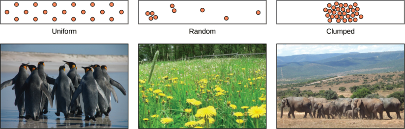
Figure \(\PageIndex{4}\): Species may have uniform, random, or clumped distribution. Territorial birds such as penguins tend to have uniform distribution. Plants such as dandelions with wind-dispersed seeds tend to be randomly distributed. Animals such as elephants that travel in groups exhibit clumped distribution (credit a: modification of work by Ben Tubby; credit b: modification of work by Rosendahl; credit c: modification of work by Rebecca Wood).

Populations distributions are limited to suitable habitats

In ecology, a niche is the match of a species to a specific environmental condition. It describes how an organism or population responds to the distribution of environmental resources (abiotic components of the environment) and predators, pathogens, and competitors (biotic components of the environment). Habitat refers to the array of resources, physical and biotic factors that are present in an area, such as to support the survival and reproduction of a particular species. The geographic range of a species can be viewed as a spatial reflection of its niche, along with characteristics of the geographic template and the species that influence its potential to colonize. The fundamental geographic range of a species is the area it occupies in which environmental conditions are favorable, without restriction from barriers to disperse or colonize (Lomolino et al 2009). A species will be confined to its realized geographic range when confronting biotic interactions or abiotic barriers that limit dispersal, a more narrow subset of its larger fundamental geographic range.

An early study on ecological niches conducted by Joseph H. Connell analyzed the environmental factors that limit the range of a barnacle (Chthamalus stellatus) on Scotland's Isle of Cumbrae (Connell 1961). In his experiments, Connell described the dominant features of C. stellatus niches and provided explanation for their distribution on intertidal zone of the rocky coast of the Isle. Connell described the upper portion of C. stellatus's range as limited by the barnacle's ability to resist dehydration during periods of low tide. The lower portion of the range was limited by interspecific interactions, namely competition with a cohabiting barnacle species and predation by a snail (Connell 1961). By removing the competing B. balanoides, Connell showed that C. stellatus was able to extend the lower edge of its realized niche in the absence of competition. These experiments demonstrate how biotic and abiotic factors limit the distribution of an organism.

 

How do populations change?

Changes in population size over time and the processes that cause these to occur are called population dynamics. How populations change in abundance over time is a major concern of population ecology, wildlife ecology, and conservation biology, and is related to questions asked in evolutionary biology. Though there are many dimensions to spatial and temporal population dynamics, discussions of population dynamics often center on changes in population size over time. Researchers who study population dynamics often use mathematical models to describe and predict population dynamics and understand what factors are driving those changes. Changes in population size are often displayed in a time series graph with time on the x-axis (usually in years) and population size (N) on the y-axis. General patterns of population dynamics in terms of population size include:

1. Growth: Growing larger than the current size (Snail kites: Figure \(\PageIndex{5}\) Panel A)
2. Decline: Decreasing in abundance (Elk: Figure \(\PageIndex{5}\) Panel B)
3. Stability: Staying approximately the same size over time (Wolves: Figure \(\PageIndex{5}\) Panel C)
4. Recovery: Stability or growth following a period of decline. (Impala: Figure \(\PageIndex{5}\) Panel D).
5. Extirpation (local extinction): Decline of one or more populations of a species to (Kirtland's Warbler, Figure \(\PageIndex{6}\) Panel A).
6. Extinction: Decline of all members of a species to (Northern White Rhino, Figure \(\PageIndex{6}\) Panel B).
7. Cycles: repeated patterns of growth followed by decline (Lynx: Figure \(\PageIndex{6}\) Panel C)

 

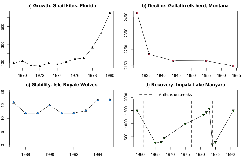
Figure \(\PageIndex{5}\):  Common patterns of population change. The x-axis in all panels is the year and the y-axis is the number of individuals.   a) Growth in a Florida Snail Kite (Rostrhamus sociabilis) population from 1970s to 1980s (Sykes 1983); b) Decline of the Gallatin, Montana herd of elk (Cervus canadensis) from the 1920s to 1960s (Peek et al. 1967); c) Stability of the Isle Royale, Michigan pack of wolves (Canis lupus) in the 1980s and 1990s (Peterson et al. 1998); d) Recovery after population crashes in the Lake Manyara National Park, Tanzania herd of impala (Prins and Weyerhaeuser 1987). 

 

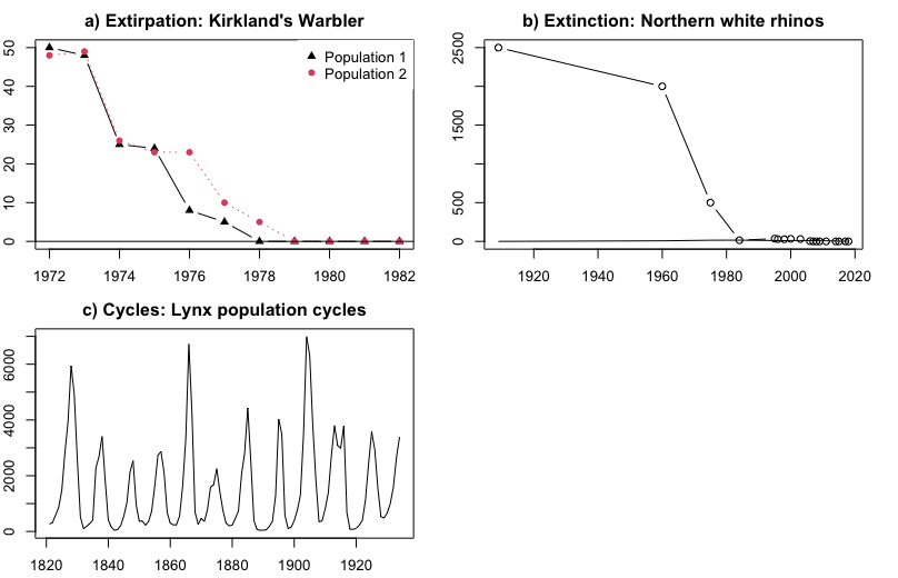
Figure \(\PageIndex{6}\):  Common patterns of population change.   The x-axis in all panels is the year. a) Decline to extirpation (local extinction) of Kirtland's Warbler in two populations (Probst 1986).  The y-axis is the number of singing males; b) Decline to global extinction of the Northern White Rhinoceros (Ceratotherium simum cottoni), one of two subspecies of White Rhinos (Smith 2001, Emslie 2012). The y-axis is the total number of rhinos in the wild. c) Repeated cycling of the Canada lynx (Lynx canadensis; Campbell and Walker 1977). The y-axis is the number of lynx trapped, an index of population size.  

Over the course of many years, a single population can display many of these dynamics.  For example, Kirtland's Warbler populations were monitored by determining the number of males defending territories in their summer breeding habitat in the Great Lakes region North America, primarily Michigan. There were about 500 males with territories in the 1950s (Figure \(\PageIndex{7}\)). The following changes occurred over the next 50 years after the species began being protected by the Endangered Species Act (Kepler et al. 1996):

1. Decline over the course of the 1960s to ~200 territories.

2. A period of stability at ~200 territories from 1975 to 1990.

3. Steady growth to >2500 from 1990 through 2020.

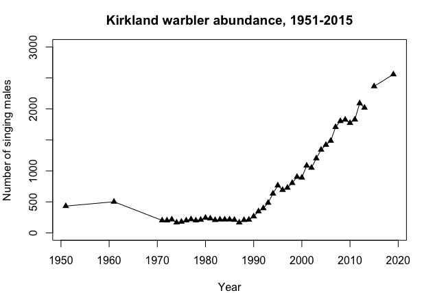
Figure \(\PageIndex{7}\):  Number of singing Kirtland's Warbler (Setophaga kirtlandii) males, 1950 to 2020.

Models can be used to understand and predict population dynamics

Researchers who study population dynamics often use mathematical models to describe and predict population dynamics and understand what factors are driving those changes. For example, if there are 2500 Kirtland’s Warblers in Michigan this year, can we predict how many will be around next year, or 10 years from now? Due to its small population size the Kirtland’s Warbler was listed as an Endangered Species in 1967. In 2019 it was de-listed and now is considered “Near-threatened.” Ecologists are very interested in using models to predict how large the Kirtland’s Warbler population will be in the future, and what factors cause it to increase and decrease (Brown et al. 2019).  In the next chapter we will explore the conceptual and mathematical tools ecologists use to understand population dynamics and predict their future trajectories.

 

Population ecologists make use of a variety of methods to model population dynamics. An accurate model should be able to describe the changes occurring in a population and predict future changes. The two simplest models of population growth use deterministic equations (equations that do not account for random events) to describe the rate of change in the size of a population over time (Figure \(\PageIndex{8}\)). The first of these models, exponential growth, describes populations that increase in numbers without any limits to their growth. The second model, logistic growth, introduces limits to reproductive growth that become more intense as the population size increases. Neither model adequately describes natural populations, but they provide points of comparison.

Figure \(\PageIndex{8}\): When resources are unlimited, populations exhibit exponential growth, resulting in a J-shaped curve. When resources are limited, populations exhibit logistic growth. In logistic growth, population expansion decreases as resources become scarce, and it levels off when the carrying capacity of the environment is reached, resulting in an S-shaped curve.

 

The Population Growth Rate (r )

The population growth rate (sometimes called the rate of increase or per capita growth rate, r) equals the birth rate (b) minus the death rate (d) divided by the initial population size (N₀).

Another method of calculating the population growth rate involves final and initial population size (figure \(\PageIndex{2}\)). In this case, population growth rate (r) equals the final population size (N) minus the initial population size (N₀) and divided by the initial population size (N₀).

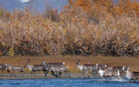
Figure \(\PageIndex{9}\): How could we calculate the growth rate of this caribou population per year if there were 200 individuals in 2016 and 300 individuals in 2018? Image by K. Joly/NPS (public domain).

 

Exponential Growth

Charles Darwin, in his theory of natural selection, was greatly influenced by the English clergyman Thomas Malthus. Malthus published a book in 1798 stating that populations with unlimited natural resources grow very rapidly, and then population growth decreases as resources become depleted. This accelerating pattern of increasing population size is called exponential growth. 

The best example of exponential growth is seen in bacteria. Bacteria are prokaryotes that reproduce quickly, about an hour for many species.  If 1000 bacteria are placed in a large flask with an unlimited supply of nutrients (so the nutrients will not become depleted), after an hour, there is one round of division and each organism divides, resulting in 2000 organisms—an increase of 1000 (Figure \(\PageIndex{10}\)). In another hour, each of the 2000 organisms will double, producing 4000, an increase of 2000 organisms. After the third hour, there should be 8000 bacteria in the flask, an increase of 4000 organisms. The important concept of exponential growth is that the population growth rate—the number of organisms added in each reproductive generation—is accelerating; that is, it is increasing at a greater and greater rate. After 1 day and 24 of these cycles, the population would have increased from 1000 to more than 16 billion. When the population size, N, is plotted over time, a J-shaped growth curve is produced (Figure \(\PageIndex{8}\)).

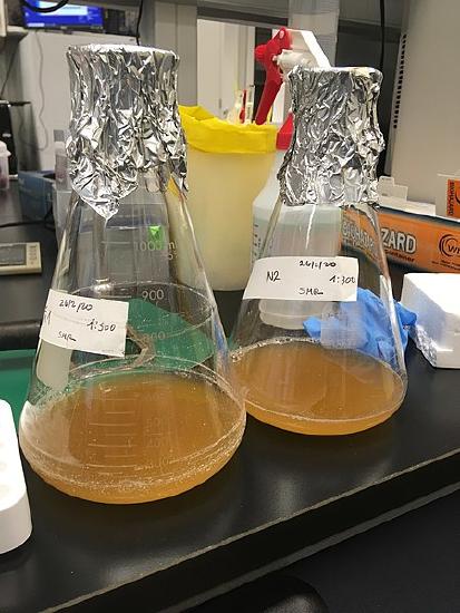
Figure \(\PageIndex{10}\): Bacteria growing with abundant nutrients in a flask will exhibit exponential growth. Image by Soledad Mirand-Rottman (CC-BY-SA).

The bacteria-in-a-flask example is not truly representative of the real world where resources are usually limited. However, when a species is introduced into a new habitat that it finds suitable, it may show exponential growth for a while. In the case of the bacteria in the flask, some bacteria will die during the experiment and thus not reproduce; therefore, the growth rate is lowered from a maximal rate in which there is no mortality.  Additionally, ecologists are interested in the population at a particular point in time, an infinitely small time interval. For this reason, the terminology of differential calculus is used to obtain the “instantaneous” growth rate, replacing the change in number and time with an instant-specific measurement of number and time.

\[\frac{d N} {d T} = bN - dN = (b - d)N \nonumber\]

Notice that the “d” associated with the first term refers to the derivative (as the term is used in calculus) and is different from the death rate, also called “\(d\).” The difference between birth and death rates is further simplified by substituting the term “r” (intrinsic rate of increase) for the relationship between birth and death rates:

\[\frac{d N} {d T} = rN \nonumber\]

The value “\(r\)” can be positive, meaning the population is increasing in size; or negative, meaning the population is decreasing in size; or zero, where the population’s size is unchanging, a condition known as zero population growth. A further refinement of the formula recognizes that different species have inherent differences in their intrinsic rate of increase (often thought of as the potential for reproduction), even under ideal conditions. Obviously, a bacterium can reproduce more rapidly and have a higher intrinsic rate of growth than a human. The maximal growth rate for a species is its biotic potential, or \(r_{max}\), thus changing the equation to:

\[\frac{d N} {d T} = r_\text{max}N \nonumber\]

Populations of all species can, potentially, increase rapidly under conditions in which resource availability and other factors are not constraining. Examples of rapid population growth are illustrated in Figure \(\PageIndex{11}\). However, unlimited growth cannot be sustained – in all of the cases in Figure \(\PageIndex{4}\), the population sizes eventually leveled off, decreased, or crashed.

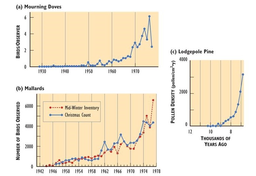
Figure \(\PageIndex{11}\): Rapid Growth of Some Natural Populations. (a) The population of mourning doves (Zenaida macroura) wintering in southern Ontario over 48 years. This used to be a rare bird, but it has apparently benefited from a warming climate, suburban habitat, and winter feeding. (b) The population of mallards (Anas platyrhynchos) wintering in southern Ontario over 35 years, illustrated with two independent sets of data. This duck has expanded its breeding and wintering ranges into eastern Canada, likely in response to habitat made available by the clearing of forest. (c) The population of lodgepole pine (Pinus contorta) near Snowshoe Lake, British Columbia, during natural afforestation following deglaciation 7000-9000 years ago. In this case, tree populations are indicated by the amount of pollen in dated layers of lake sediment. Sources: Modified from (a) Freedman and Riley (1980); (b) Goodwin et al. (1977); (c) MacDonald and Cwynar (1991).

Logistic Growth

Exponential growth is possible only when infinite natural resources are available; this is not the case in the real world. Charles Darwin recognized this fact in his description of the “struggle for existence,” which states that individuals will compete (with members of their own or other species) for limited resources. The successful ones will survive to pass on their own characteristics and traits (which we know now are transferred by genes) to the next generation at a greater rate (natural selection). To model the reality of limited resources, population ecologists developed the logistic growth model.

In the real world, with its limited resources, exponential growth cannot continue indefinitely. Exponential growth may occur in environments where there are few individuals and plentiful resources, but when the number of individuals gets large enough, resources will be depleted, slowing the growth rate. Eventually, the growth rate will plateau or level off (Figure \(\PageIndex{8 and 12}\)). This population size, which represents the maximum population size that a particular environment can support, is called the carrying capacity, or \(K\).  There are three different sections to an S-shaped curve. Initially, growth is exponential because there are few individuals and ample resources available. Then, as resources begin to become limited, the growth rate decreases. Finally, growth levels off at the carrying capacity of the environment, with little change in population size over time.

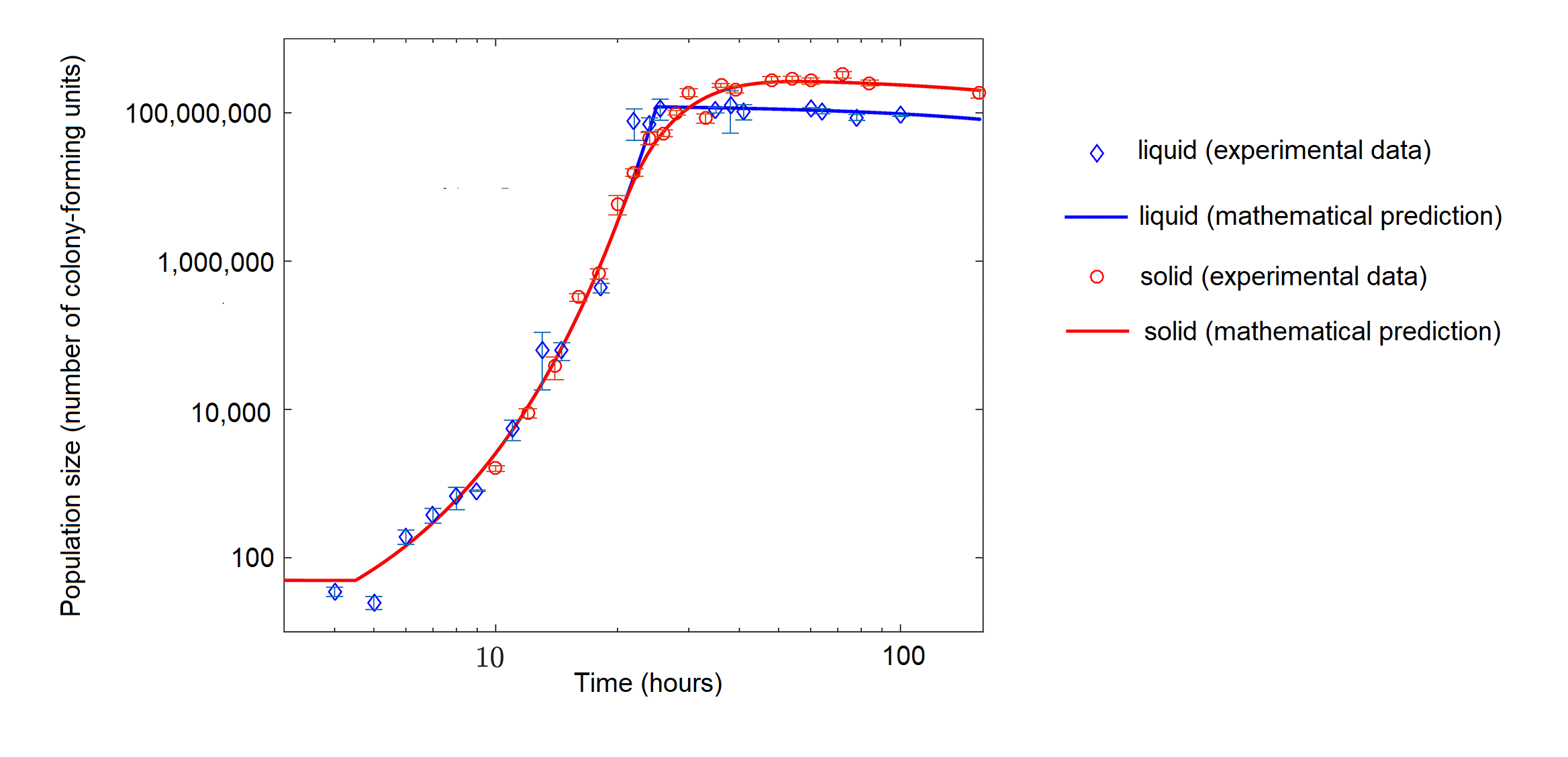
Figure \(\PageIndex{12}\): The growth of the bacterium Escherichia coli (E. coli) with limited nutrients over time in hours. Population size is in number of colony-forming units, which is a cell capable of dividing to produce a colony of cells. The bacteria were grown in liquid (blue diamonds) or on a semisolid medium (agar, red circles). The points represent actual measurements of populations size, and the lines represent a mathematical model, basically a prediction that is based on the data points. The data show logistic population growth, particularly in solid media. Initially, population size increases rapidly (concave part of curve), but the growth rate then stabilizes (straight line) before decreasing (convex part of curve) and leveling near the carrying capacity. Image modified from Shao X, Mugler A, Kim J, Jeong HJ, Levin BR, Nemenman I (2017) Growth of bacteria in 3-d colonies. PLoS Comput Biol 13(7): e1005679 (CC-BY).

In some populations, there are variations to the S-shaped curve. Examples in wild populations include sheep and harbor seals (figure \(\PageIndex{13}\)). In both examples, the population size exceeds the carrying capacity for short periods of time and then falls below the carrying capacity afterwards. This fluctuation in population size continues to occur as the population oscillates around its carrying capacity. Still, even with this oscillation the logistic model is confirmed.

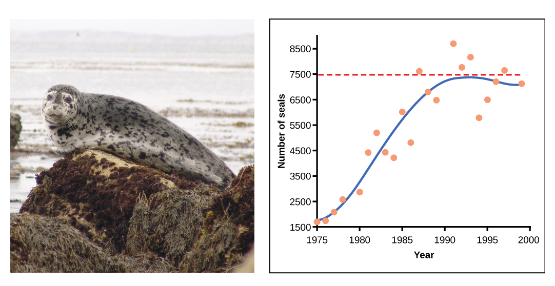
Figure \(\PageIndex{13}\): A natural population of seals shows logistic growth. The number of seals, ranging from 1500 to 8500, is on the y-axis, and the year, ranging from 1975-2000, is on the x-axis. Orange dots represent the observed population size each year, and the blue line represent the trend. From 1975 to 1983, the blue line curves upwards, representing an increase in both population size and population growth rate. From 1983 to 1992, the curve flattens, representing that population size is still increasing, but population growth rate is decreasing. After 1992, population fluctuates near the carrying capacity (dotted, horizontal line). 

The formula we use to calculate logistic growth adds the carrying capacity as a moderating force in the growth rate. The expression “\(K – N\)” is indicative of how many individuals may be added to a population at a given stage, and “\(K – N\)” divided by “\(K\)” is the fraction of the carrying capacity available for further growth. Thus, the exponential growth model is restricted by this factor to generate the logistic growth equation:

\[\begin{align} \dfrac{d N} {d T}
&= r_\text{max} \frac{d N} {d T} \nonumber \\[5pt]
&= r_\text{max}N \frac{(K-N)} {K}\nonumber
\end{align} \nonumber\]

Notice that when \(N\) is very small, \((K-N)/K\) becomes close to \(K/K\) or \(1\), and the right side of the equation reduces to \(r_{max}N\), which means the population is growing exponentially and is not influenced by carrying capacity. On the other hand, when \(N\) is large, \((K-N)/K\) come close to zero, which means that population growth will be slowed greatly or even stopped. Thus, population growth is greatly slowed in large populations by the carrying capacity \(K\). This model also allows for the population of a negative population growth, or a population decline. This occurs when the number of individuals in the population exceeds the carrying capacity (because the value of \((K-N)/K\) is negative).

The logistic model assumes that every individual within a population will have equal access to resources and, thus, an equal chance for survival. For plants, the amount of water, sunlight, nutrients, and the space to grow are the important resources, whereas in animals, important resources include food, water, shelter, nesting space, and mates.  In the real world, phenotypic variation among individuals within a population means that some individuals will be better adapted to their environment than others. The resulting competition between population members of the same species for resources is termed intraspecific competition (intra- = “within”; -specific = “species”). Intraspecific competition for resources may not affect populations that are well below their carrying capacity—resources are plentiful and all individuals can obtain what they need. However, as population size increases, this competition intensifies. In addition, the accumulation of waste products can reduce an environment’s carrying capacity.  

The logistic population growth model is not the only way that populations respond to limited resources. In some populations, growth is exponential until resources run low, wastes accumulate, or disease spreads (see limiting factors below), and the population then crashes (Figure \(\PageIndex{14}\)). Thus, population growth rate (and size) may plummet rapidly instead of tapering as it approaches the carrying capacity. 

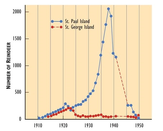
Figure \(\PageIndex{14}\):  Population Growth and Crash. In 1910, reindeer (Rangifer tarandus tarandus; the Eurasian subspecies of caribou) were introduced to two islands in the Aleutian chain off Alaska in an attempt to establish a new food resource for local use. On both islands, the reindeer population increased rapidly. However, they exceeded the carrying capacity of the habitat and caused severe damage through overgrazing. The populations then crashed. Source: Modified from Krebs (1985).

 

Factors that Regulate Population Growth

The logistic model of population growth, while valid in many natural populations and a useful model, is a simplification of real-world population dynamics. Implicit in the model is that the carrying capacity of the environment does not change, which is not the case. The carrying capacity varies annually: for example, some summers are hot and dry whereas others are cold and wet. In many areas, the carrying capacity during the winter is much lower than it is during the summer. Also, natural events such as earthquakes, volcanoes, and fires can alter an environment and hence its carrying capacity. Additionally, populations do not usually exist in isolation. They engage in interspecific competition: that is, they share the environment with other species, competing with them for the same resources. These factors are also important to understanding how a specific population will grow.

Nature regulates population growth in a variety of ways. These are grouped into density-dependent factors, in which the density of the population at a given time affects growth rate and mortality, and density-independent factors, which influence mortality in a population regardless of population density. Note that in the former, the effect of the factor on the population depends on the density of the population at onset. Conservation biologists want to understand both types because this helps them manage populations and prevent extinction or overpopulation.

Density-dependent Regulation

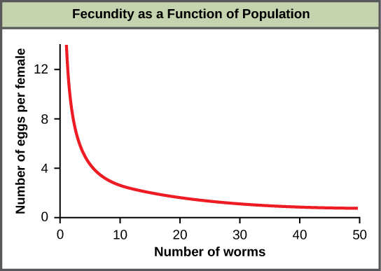
Most density-dependent factors are biological in nature (biotic). Usually, the denser a population is, the greater its mortality rate. Density-dependent factors include predation, parasitism, herbivory, competition, and accumulation of waste. An example of density-dependent regulation is shown in figure \(\PageIndex{15}\) with results from a study focusing on the giant intestinal roundworm (Ascaris lumbricoides), a parasite of humans and other mammals. Denser populations of the parasite exhibited lower fecundity: they contained fewer eggs. One possible explanation for this is that females would be smaller in more dense populations (due to limited resources) and that smaller females would have fewer eggs. This hypothesis was tested and disproved in a 2009 study which showed that female weight had no influence. The actual cause of the density-dependence of fecundity in this organism is still unclear and awaiting further investigation.

Figure \(\PageIndex{15}\): In this population of roundworms, fecundity (number of eggs) decreases with population density.³

As a population increases, its predators are able to harvest it more easily. Prey density also affects population growth rate of predators: low prey density increases the mortality of its predator because it has more difficulty locating its food sources.  Parasites are able to pass from host to host more easily as the population density of the host increases. For this reason, epidemics among humans are particularly severe in cities. In fact, for most of the period since humans began living in cities, city populations have been maintained only through continual immigration from the countryside. Not until the development of community sanitation, immunization, and other public health measures did cities avoid periodic sharp drops in population as a result of epidemics. The recurrent epidemics of the "black death" in Europe that began in the fourteenth century caused a sharp decline in population. In just three years (1348–1350), at least one-quarter of the population of Europe died from the disease (probably plague). Similarly, herbivores can more easily spread between individual plants in a dense population. This is why strip cropping helps control pests. An herbivore or plant pathogen may infect one row of plants, but it is less likely to spread to more distant rows of that species.

Intraspecific competition (and interspecific competition) can be important density dependent factors. In the summer of 1980, much of southern New England was struck by an infestation of the gypsy moth (figure \(\PageIndex{16}\)). As the summer wore on, the larvae (caterpillars) pupated, the hatched adults mated, the females laid masses of eggs (each mass containing several hundred eggs) on virtually every tree in the region. In early May of 1981, the young caterpillars that hatched from these eggs began feeding and molting.  In 72 hours, a 50-ft beech tree or a 25-ft white pine tree would be completely defoliated. Large patches of forest began to take on a winter appearance with their skeletons of bare branches. In fact, the infestation was so heavy that many trees were completely defoliated before the caterpillars could complete their larval development. The result: a massive die-off of the animals; very few succeeded in completing metamorphosis. Here, then, was a dramatic example of how competition among members of one species for a finite resource - in this case, food - caused a sharp drop in population. The effect was clearly density-dependent. The lower population densities of the previous summer had permitted most of the animals to complete their life cycle.

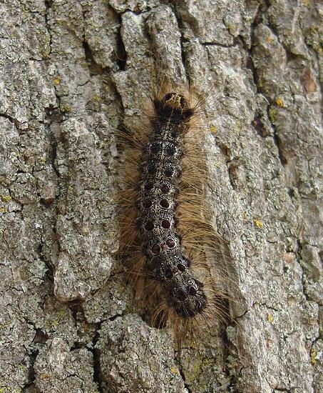
Figure \(\PageIndex{16}\): Gypsy moth caterpillars face intraspecific competition at high densities. Image by Editor at Large (CC-BY-SA).  

Density-independent Regulation

Many factors, typically physical or chemical in nature (abiotic), influence the mortality of a population regardless of its density, including weather, natural disasters, and pollution (Figure \(\PageIndex{17}\)). An individual deer may be killed in a forest fire regardless of how many deer happen to be in that area. Its chances of survival are the same whether the population density is high or low. The same holds true for cold winter weather.  Not only do abiotic factors limit population growth but they often drive existing populations well below their previous level.

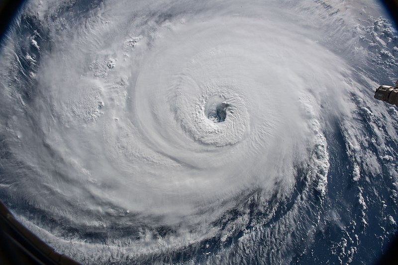
Figure \(\PageIndex{17}\): Severe weather, like Hurricane Florence of 2018, can reduce population size regardless of density. Image by NASA Goddard Space Flight Center (CC-BY)

These factors are described as density-independent because they exert their effect irrespective of the size of the population when the catastrophe struck.  This graph (Figure \(\PageIndex{18}\), from P. T. Boag and P.R. Grant in Science, 214:82, 1981) shows the decline in the population of one of Darwin's finches (Geospiza fortis) on Daphne Major, a tiny (100 acres = 40 hectares) member of the Galapagos Islands. The decline (from 1400 to 200 individuals) occurred because of a severe drought that reduced the quantity of seeds on which this species feeds. The drought ended in 1978, but even with ample food once again available the finch population recovered only slowly.

Figure \(\PageIndex{17}\): Left: This graph (from P. T. Boag and P.R. Grant in Science, 214:82, 1981) shows the decline in the population of one of Darwin's finches (Geospiza fortis) on Daphne Major, a tiny (100 acres = 40 hectares) member of the Galapagos Islands. The decline (from 1400 to 200 individuals) occurred because of a severe drought that reduced the quantity of seeds on which this species feeds.  Right: The graph (redrawn from R. H. MacArthur and E. O. Wilson, The Theory of Island Biogeography, Princeton University Press) shows the number of species of reptiles and amphibians on various islands in the West Indies.

In real-life situations, population regulation is very complicated and density-dependent and independent factors can interact. A dense population that is reduced in a density-independent manner by some environmental factor(s) will be able to recover differently than a sparse population. For example, a population of deer affected by a harsh winter will recover faster if there are more deer remaining to reproduce.

Catastrophic declines are particularly risky for populations living on islands. The smaller the island, the smaller the population of each species on it, and the greater the risk that a catastrophe will so decimate the population that it becomes extinct. This appears to be one reason for the clear relationship between size of island and the number of different species it contains.  The graph (Figure \(\PageIndex{17}\), redrawn from R. H. MacArthur and E. O. Wilson, The Theory of Island Biogeography, Princeton University Press) shows the number of species of reptiles and amphibians on various islands in the West Indies. In general, if one island has 10 times the area of another, it will contain approximately twice the number of species.  The same principle applies to many habitats. In a sense, most habitats are islands. A series of ponds, a range of mountain tops, scattered groves of citrus trees, even individual trees within a grove, all are made up of patches of habitat separated by barriers to the free migration of their inhabitants.

This has practical as well as theoretical importance. As the human population grows, jungles are cleared for agriculture, farms are paved for shopping centers, rivers are dammed for hydroelectric power and irrigation, etc. Although wildlife sanctuaries are being established, they must be made large enough so that they can support populations large enough to survive density-independent checks when they strike.

Demography

Demography is the statistical study of population changes over time: birth rates, death rates, and life expectancies. Each of these measures, especially birth rates, may be affected by the population characteristics described above. For example, a large population size results in a higher birth rate because more potentially reproductive individuals are present. In contrast, a large population size can also result in a higher death rate because of competition, disease, and the accumulation of waste. Similarly, a higher population density or a clumped dispersion pattern results in more potential reproductive encounters between individuals, which can increase birth rate. Lastly, a female-biased sex ratio (the ratio of males to females) or age structure (the proportion of population members at specific age ranges) composed of many individuals of reproductive age can increase birth rates. In addition, the demographic characteristics of a population can influence how the population grows or declines over time. If birth and death rates are equal, the population remains stable. However, the population size will increase if birth rates exceed death rates; the population will decrease if birth rates are less than death rates. Life expectancy is another important factor; the length of time individuals remain in the population impacts local resources, reproduction, and the overall health of the population. These demographic characteristics are often displayed in the form of a life table.

Life tables provide important information about the life history of an organism. Life tables divide the population into age groups and often sexes, and show how long a member of that group is likely to live. They are modeled after actuarial tables used by the insurance industry for estimating human life expectancy. Life tables may include the probability of individuals dying before their next birthday (i.e., their mortality rate), the percentage of surviving individuals dying at a particular age interval, and their life expectancy at each interval. An example of a life table is shown in Table \(\PageIndex{1}\) from a study of Dall mountain sheep, a species native to northwestern North America. Notice that the population is divided into age intervals (column A). The mortality rate (per ), shown in column D, is based on the number of individuals dying during the age interval (column B) divided by the number of individuals surviving at the beginning of the interval (Column C), multiplied by .

\[\text{mortality rate} = \frac{\text{number of individuals dying}} {\text{number of individuals surviving}} * 1000 \nonumber\]

For example, between ages three and four, 12 individuals die out of the 776 that were remaining from the original 1000 sheep. This number is then multiplied by 1000 to get the mortality rate per thousand.

\[\text{mortality rate} = \frac{12} {776} * 1000 \approx 15.5 \nonumber\]

As can be seen from the mortality rate data (column D), a high death rate occurred when the sheep were between 6 and 12 months old, and then increased even more from 8 to 12 years old, after which there were few survivors. The data indicate that if a sheep in this population were to survive to age one, it could be expected to live another 7.7 years on average, as shown by the life expectancy numbers in column E.

 

Table \(\PageIndex{1}\): Life Table of Dall Mountain Sheep¹

Age interval (years)	Number dying in age interval out of 1000 born	Number surviving at beginning of age interval out of 1000 born	Mortality rate per 1000 alive at beginning of age interval	Life expectancy or mean lifetime remaining to those attaining age interval
0-0.5	54	1000	54.0	7.06
0.5-1	145	946	153.3	--
1-2	12	801	15.0	7.7
2-3	13	789	16.5	6.8
3-4	12	776	15.5	5.9
4-5	30	764	39.3	5.0
5-6	46	734	62.7	4.2
6-7	48	688	69.8	3.4
7-8	69	640	107.8	2.6
8-9	132	571	231.2	1.9
9-10	187	439	426.0	1.3
10-11	156	252	619.0	0.9
11-12	90	96	937.5	0.6
12-13	3	6	500.0	1.2
13-14	3	3	1000	0.7

 

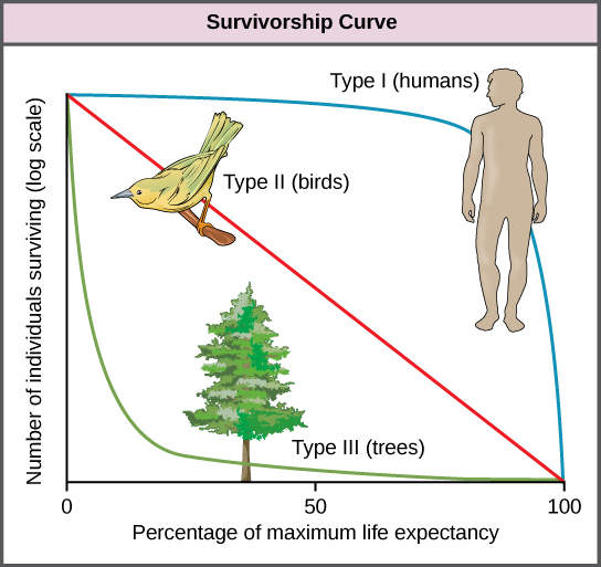
Another tool used by population ecologists is a survivorship curve, which is a graph of the number of individuals surviving at each age interval plotted versus time (usually with data compiled from a life table). These curves allow us to compare the life histories of different populations (Figure \(\PageIndex{18}\)). Humans and most primates exhibit a Type I survivorship curve because a high percentage of offspring survive their early and middle years—death occurs predominantly in older individuals. These types of species usually have small numbers of offspring at one time, and they give a high amount of parental care to them to ensure their survival. Birds are an example of an intermediate or Type II survivorship curve because birds die more or less equally at each age interval. These organisms also may have relatively few offspring and provide significant parental care. Trees, marine invertebrates, and most fishes exhibit a Type III survivorship curve because very few of these organisms survive their younger years; however, those that make it to an old age are more likely to survive for a relatively long period of time. Organisms in this category usually have a very large number of offspring, but once they are born, little parental care is provided. Thus these offspring are “on their own” and vulnerable to predation, but their sheer numbers assure the survival of enough individuals to perpetuate the species.

 

Figure \(\PageIndex{18}\): Survivorship curves show the distribution of individuals in a population according to age. Humans and most mammals have a Type I survivorship curve because death primarily occurs in the older years. Birds have a Type II survivorship curve, as death at any age is equally probable. Trees have a Type III survivorship curve because very few survive the younger years, but after a certain age, individuals are much more likely to survive.

Life History Patterns and Energy Budgets

Energy is required by all living organisms for their growth, maintenance, and reproduction; at the same time, energy is often a major limiting factor in determining an organism’s survival. Plants, for example, acquire energy from the sun via photosynthesis, but must expend this energy to grow, maintain health, and produce energy-rich seeds to produce the next generation. Animals have the additional burden of using some of their energy reserves to acquire food. Furthermore, some animals must expend energy caring for their offspring. Thus, all species have an energy budget: they must balance energy intake with their use of energy for metabolism, reproduction, parental care, and energy storage (such as bears building up body fat for winter hibernation).

Parental Care and Fecundity

Fecundity is the potential reproductive capacity of an individual within a population. In other words, fecundity describes how many offspring could ideally be produced if an individual has as many offspring as possible, repeating the reproductive cycle as soon as possible after the birth of the offspring. In animals, fecundity is inversely related to the amount of parental care given to an individual offspring. Species, such as many marine invertebrates, that produce many offspring usually provide little if any care for the offspring (they would not have the energy or the ability to do so anyway). Most of their energy budget is used to produce many tiny offspring. Animals with this strategy are often self-sufficient at a very early age. This is because of the energy tradeoff these organisms have made to maximize their evolutionary fitness. Because their energy is used for producing offspring instead of parental care, it makes sense that these offspring have some ability to be able to move within their environment and find food and perhaps shelter. Even with these abilities, their small size makes them extremely vulnerable to predation, so the production of many offspring allows enough of them to survive to maintain the species.

Animal species that have few offspring during a reproductive event usually give extensive parental care, devoting much of their energy budget to these activities, sometimes at the expense of their own health. This is the case with many mammals, such as humans, kangaroos, and pandas. The offspring of these species are relatively helpless at birth and need to develop before they achieve self-sufficiency.

Plants with low fecundity produce few energy-rich seeds (such as coconuts and chestnuts) with each having a good chance to germinate into a new organism; plants with high fecundity usually have many small, energy-poor seeds (like orchids) that have a relatively poor chance of surviving. Although it may seem that coconuts and chestnuts have a better chance of surviving, the energy tradeoff of the orchid is also very effective. It is a matter of where the energy is used, for large numbers of seeds or for fewer seeds with more energy.

Early versus Late Reproduction

The timing of reproduction in a life history also affects species survival. Organisms that reproduce at an early age have a greater chance of producing offspring, but this is usually at the expense of their growth and the maintenance of their health. Conversely, organisms that start reproducing later in life often have greater fecundity or are better able to provide parental care, but they risk that they will not survive to reproductive age. Examples of this can be seen in fishes. Small fish like guppies use their energy to reproduce rapidly, but never attain the size that would give them defense against some predators. Larger fish, like the bluegill or shark, use their energy to attain a large size, but do so with the risk that they will die before they can reproduce or at least reproduce to their maximum. These different energy strategies and tradeoffs are key to understanding the evolution of each species as it maximizes its fitness and fills its niche. In terms of energy budgeting, some species “blow it all” and use up most of their energy reserves to reproduce early before they die. Other species delay having reproduction to become stronger, more experienced individuals and to make sure that they are strong enough to provide parental care if necessary.

Single versus Multiple Reproductive Events

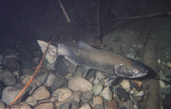
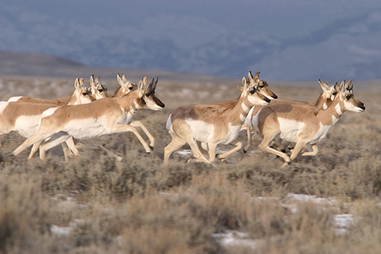
Some life history traits, such as fecundity, timing of reproduction, and parental care, can be grouped together into general strategies that are used by multiple species. Semelparity occurs when a species reproduces only once during its lifetime and then dies. Such species use most of their resource budget during a single reproductive event, sacrificing their health to the point that they do not survive. Examples of semelparity are bamboo, which flowers once and then dies, and the Chinook salmon (Figure \(\PageIndex{19}\)a), which uses most of its energy reserves to migrate from the ocean to its freshwater nesting area, where it reproduces and then dies. Scientists have posited alternate explanations for the evolutionary advantage of the Chinook’s post-reproduction death: a programmed suicide caused by a massive release of corticosteroid hormones, presumably so the parents can become food for the offspring, or simple exhaustion caused by the energy demands of reproduction; these are still being debated.

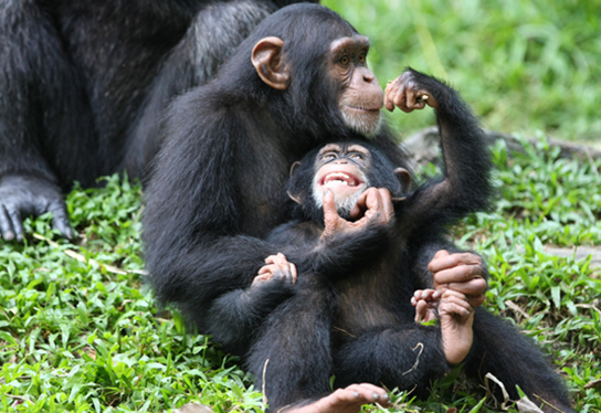
Iteroparity describes species that reproduce repeatedly during their lives. Some animals are able to mate only once per year, but survive multiple mating seasons. The pronghorn antelope is an example of an animal that goes into a seasonal estrus cycle (“heat”): a hormonally induced physiological condition preparing the body for successful mating (Figure \(\PageIndex{19}\)b). Females of these species mate only during the estrus phase of the cycle. A different pattern is observed in primates, including humans and chimpanzees, which may attempt reproduction at any time during their reproductive years, even though their menstrual cycles make pregnancy likely only a few days per month during ovulation (Figure \(\PageIndex{19}\)c).

a

b

c

Figure \(\PageIndex{19}\): The (a) Chinook salmon mates once and dies. The (b) pronghorn antelope mates during specific times of the year during its reproductive life. Primates, such as humans and (c) chimpanzees, may mate on any day, independent of ovulation. (credit a: modification of work by Roger Tabor, USFWS; credit b: modification of work by Mark Gocke, USDA; credit c: modification of work by “Shiny Things”/Flickr)

 

References

• Data Adapted from Edward S. Deevey, Jr., “Life Tables for Natural Populations of Animals,” The Quarterly Review of Biology 22, no. 4 (December 1947): 283-314.
• Adapted from Phillip G. Byrne and William R. Rice, “Evidence for adaptive male mate choice in the fruit fly Drosophila melanogaster,” Proc Biol Sci. 273, no. 1589 (2006): 917-922, doi: 10.1098/rspb.2005.3372.
• N.A. Croll et al., “The Population Biology and Control of Ascaris lumbricoides in a Rural Community in Iran.” Transactions of the Royal Society of Tropical Medicine and Hygiene 76, no. 2 (1982): 187-197, doi:10.1016/0035-9203(82)90272-3.
• Martin Walker et al., “Density-Dependent Effects on the Weight of Female Ascaris lumbricoides Infections of Humans and its Impact on Patterns of Egg Production.” Parasites & Vectors 2, no. 11 (February 2009), doi:10.1186/1756-3305-2-11.
• David Nogués-Bravo et al., “Climate Change, Humans, and the Extinction of the Woolly Mammoth.” PLoS Biol 6 (April 2008): e79, doi:10.1371/journal.pbio.0060079.
• G.M. MacDonald et al., “Pattern of Extinction of the Woolly Mammoth in Beringia.” Nature Communications 3, no. 893 (June 2012), doi:10.1038/ncomms1881.
• Freedman, B. and J. Riley. 1980. Population trends of various species of birds wintering in southern Ontario. Ontario Field Biologist, 34: 49-79.
• Goodwin, C. E., B. Freedman, and S. M. McKay. 1977. Population trends in waterfowl wintering in the Toronto region, 1929–1976. Ontario Field Biologist, 31: 1-28.
• Krebs, C.J. 2008. Ecology: The Experimental Analysis of Distribution and Abundance. 6th ed. Benjamin Cummings, New York, NY.
• MacDonald, G.M. and L.C. Cwynar. 1991. Post-glacial population growth rates of Pinus contorta ssp. latifolia in western Canada. Journal of Ecology, 79: 417-429.

 

Contributors and Attributions

This chapter was written by N. Brouwer and K. Whittinghill with text taken from the following CC-BY resources:

• Ecological niche by Wikipedia, the free encyclopedia
• OpenStax Biology e section . Population Demography
• OpenStax Biology e section . Population Dynamics and Regulation
• .: Population Dynamics and Regulation by OpenStax, is licensed CC BY by

  Connie Rye (East Mississippi Community College), Robert Wise (University of Wisconsin, Oshkosh), Vladimir Jurukovski (Suffolk County Community College), Jean DeSaix (University of North Carolina at Chapel Hill), Jung Choi (Georgia Institute of Technology), Yael Avissar (Rhode Island College) among other contributing authors. Original content by OpenStax (CC BY 4.0; Download for free at http://cnx.org/contents/185cbf87-c72...f21b5eabd@9.87).

• .: Environmental Limits to Population Growth by OpenStax, is licensed CC BY by

  Connie Rye (East Mississippi Community College), Robert Wise (University of Wisconsin, Oshkosh), Vladimir Jurukovski (Suffolk County Community College), Jean DeSaix (University of North Carolina at Chapel Hill), Jung Choi (Georgia Institute of Technology), Yael Avissar (Rhode Island College) among other contributing authors. Original content by OpenStax (CC BY 4.0; Download for free at http://cnx.org/contents/185cbf87-c72...f21b5eabd@9.87).

• .B: Principles of Population Growth by John W. Kimball, is licensed CC BY. This content is distributed under a Creative Commons Attribution . Unported (CC BY .) license and made possible by funding from The Saylor Foundation
• Population Growth and Regulation from Environmental Biology by Matthew R. Fisher (CC-BY)
• Principles of Population Growth and The Human Population from Biology by John W. Kimball (CC-BY)
• Ecology: From Individuals to the Biosphere in Environmental Science: A Canadian Perspective by Bill Freedman
• Population Demography and Life Histories and Natural Selection by OpenStax, is licensed CC BY by

  Connie Rye (East Mississippi Community College), Robert Wise (University of Wisconsin, Oshkosh), Vladimir Jurukovski (Suffolk County Community College), Jean DeSaix (University of North Carolina at Chapel Hill), Jung Choi (Georgia Institute of Technology), Yael Avissar (Rhode Island College) among other contributing authors. Original content by OpenStax (CC BY 4.0; Download for free at http://cnx.org/contents/185cbf87-c72...f21b5eabd@9.87).

• Population Demographics and Dynamics from Environmental Biology by Matthew R. Fisher (CC-BY)
• Population Demography and Life Histories and Natural Selection by OpenStax, is licensed CC BY by

  Connie Rye (East Mississippi Community College), Robert Wise (University of Wisconsin, Oshkosh), Vladimir Jurukovski (Suffolk County Community College), Jean DeSaix (University of North Carolina at Chapel Hill), Jung Choi (Georgia Institute of Technology), Yael Avissar (Rhode Island College) among other contributing authors. Original content by OpenStax (CC BY 4.0; Download for free at http://cnx.org/contents/185cbf87-c72...f21b5eabd@9.87).

• Population Dynamics and Regulation from General Biology by OpenStax (CC-BY)
• Population Demographics and Dynamics from Environmental Biology by Matthew R. Fisher (CC-BY)
• Principles of Population Growth from Biology by John W. Kimball (CC-BY)