10.3: Pre-lab Questions
- Page ID
- 40213
\( \newcommand{\vecs}[1]{\overset { \scriptstyle \rightharpoonup} {\mathbf{#1}} } \)
\( \newcommand{\vecd}[1]{\overset{-\!-\!\rightharpoonup}{\vphantom{a}\smash {#1}}} \)
\( \newcommand{\dsum}{\displaystyle\sum\limits} \)
\( \newcommand{\dint}{\displaystyle\int\limits} \)
\( \newcommand{\dlim}{\displaystyle\lim\limits} \)
\( \newcommand{\id}{\mathrm{id}}\) \( \newcommand{\Span}{\mathrm{span}}\)
( \newcommand{\kernel}{\mathrm{null}\,}\) \( \newcommand{\range}{\mathrm{range}\,}\)
\( \newcommand{\RealPart}{\mathrm{Re}}\) \( \newcommand{\ImaginaryPart}{\mathrm{Im}}\)
\( \newcommand{\Argument}{\mathrm{Arg}}\) \( \newcommand{\norm}[1]{\| #1 \|}\)
\( \newcommand{\inner}[2]{\langle #1, #2 \rangle}\)
\( \newcommand{\Span}{\mathrm{span}}\)
\( \newcommand{\id}{\mathrm{id}}\)
\( \newcommand{\Span}{\mathrm{span}}\)
\( \newcommand{\kernel}{\mathrm{null}\,}\)
\( \newcommand{\range}{\mathrm{range}\,}\)
\( \newcommand{\RealPart}{\mathrm{Re}}\)
\( \newcommand{\ImaginaryPart}{\mathrm{Im}}\)
\( \newcommand{\Argument}{\mathrm{Arg}}\)
\( \newcommand{\norm}[1]{\| #1 \|}\)
\( \newcommand{\inner}[2]{\langle #1, #2 \rangle}\)
\( \newcommand{\Span}{\mathrm{span}}\) \( \newcommand{\AA}{\unicode[.8,0]{x212B}}\)
\( \newcommand{\vectorA}[1]{\vec{#1}} % arrow\)
\( \newcommand{\vectorAt}[1]{\vec{\text{#1}}} % arrow\)
\( \newcommand{\vectorB}[1]{\overset { \scriptstyle \rightharpoonup} {\mathbf{#1}} } \)
\( \newcommand{\vectorC}[1]{\textbf{#1}} \)
\( \newcommand{\vectorD}[1]{\overrightarrow{#1}} \)
\( \newcommand{\vectorDt}[1]{\overrightarrow{\text{#1}}} \)
\( \newcommand{\vectE}[1]{\overset{-\!-\!\rightharpoonup}{\vphantom{a}\smash{\mathbf {#1}}}} \)
\( \newcommand{\vecs}[1]{\overset { \scriptstyle \rightharpoonup} {\mathbf{#1}} } \)
\(\newcommand{\longvect}{\overrightarrow}\)
\( \newcommand{\vecd}[1]{\overset{-\!-\!\rightharpoonup}{\vphantom{a}\smash {#1}}} \)
\(\newcommand{\avec}{\mathbf a}\) \(\newcommand{\bvec}{\mathbf b}\) \(\newcommand{\cvec}{\mathbf c}\) \(\newcommand{\dvec}{\mathbf d}\) \(\newcommand{\dtil}{\widetilde{\mathbf d}}\) \(\newcommand{\evec}{\mathbf e}\) \(\newcommand{\fvec}{\mathbf f}\) \(\newcommand{\nvec}{\mathbf n}\) \(\newcommand{\pvec}{\mathbf p}\) \(\newcommand{\qvec}{\mathbf q}\) \(\newcommand{\svec}{\mathbf s}\) \(\newcommand{\tvec}{\mathbf t}\) \(\newcommand{\uvec}{\mathbf u}\) \(\newcommand{\vvec}{\mathbf v}\) \(\newcommand{\wvec}{\mathbf w}\) \(\newcommand{\xvec}{\mathbf x}\) \(\newcommand{\yvec}{\mathbf y}\) \(\newcommand{\zvec}{\mathbf z}\) \(\newcommand{\rvec}{\mathbf r}\) \(\newcommand{\mvec}{\mathbf m}\) \(\newcommand{\zerovec}{\mathbf 0}\) \(\newcommand{\onevec}{\mathbf 1}\) \(\newcommand{\real}{\mathbb R}\) \(\newcommand{\twovec}[2]{\left[\begin{array}{r}#1 \\ #2 \end{array}\right]}\) \(\newcommand{\ctwovec}[2]{\left[\begin{array}{c}#1 \\ #2 \end{array}\right]}\) \(\newcommand{\threevec}[3]{\left[\begin{array}{r}#1 \\ #2 \\ #3 \end{array}\right]}\) \(\newcommand{\cthreevec}[3]{\left[\begin{array}{c}#1 \\ #2 \\ #3 \end{array}\right]}\) \(\newcommand{\fourvec}[4]{\left[\begin{array}{r}#1 \\ #2 \\ #3 \\ #4 \end{array}\right]}\) \(\newcommand{\cfourvec}[4]{\left[\begin{array}{c}#1 \\ #2 \\ #3 \\ #4 \end{array}\right]}\) \(\newcommand{\fivevec}[5]{\left[\begin{array}{r}#1 \\ #2 \\ #3 \\ #4 \\ #5 \\ \end{array}\right]}\) \(\newcommand{\cfivevec}[5]{\left[\begin{array}{c}#1 \\ #2 \\ #3 \\ #4 \\ #5 \\ \end{array}\right]}\) \(\newcommand{\mattwo}[4]{\left[\begin{array}{rr}#1 \amp #2 \\ #3 \amp #4 \\ \end{array}\right]}\) \(\newcommand{\laspan}[1]{\text{Span}\{#1\}}\) \(\newcommand{\bcal}{\cal B}\) \(\newcommand{\ccal}{\cal C}\) \(\newcommand{\scal}{\cal S}\) \(\newcommand{\wcal}{\cal W}\) \(\newcommand{\ecal}{\cal E}\) \(\newcommand{\coords}[2]{\left\{#1\right\}_{#2}}\) \(\newcommand{\gray}[1]{\color{gray}{#1}}\) \(\newcommand{\lgray}[1]{\color{lightgray}{#1}}\) \(\newcommand{\rank}{\operatorname{rank}}\) \(\newcommand{\row}{\text{Row}}\) \(\newcommand{\col}{\text{Col}}\) \(\renewcommand{\row}{\text{Row}}\) \(\newcommand{\nul}{\text{Nul}}\) \(\newcommand{\var}{\text{Var}}\) \(\newcommand{\corr}{\text{corr}}\) \(\newcommand{\len}[1]{\left|#1\right|}\) \(\newcommand{\bbar}{\overline{\bvec}}\) \(\newcommand{\bhat}{\widehat{\bvec}}\) \(\newcommand{\bperp}{\bvec^\perp}\) \(\newcommand{\xhat}{\widehat{\xvec}}\) \(\newcommand{\vhat}{\widehat{\vvec}}\) \(\newcommand{\uhat}{\widehat{\uvec}}\) \(\newcommand{\what}{\widehat{\wvec}}\) \(\newcommand{\Sighat}{\widehat{\Sigma}}\) \(\newcommand{\lt}{<}\) \(\newcommand{\gt}{>}\) \(\newcommand{\amp}{&}\) \(\definecolor{fillinmathshade}{gray}{0.9}\)- What is meant by “serial dilution”?
- Why would it be important to know the number of bacteria in a food or beverage sample?
- Write the following in scientific notation:
- 1:10
- 1:10,000
- 234 x 104
- What is the inverse of 3.0 x 10⁻⁵?
- Which methods might over estimate the number of cells in a sample?
- The Direct Count
- The Standard Plate Count-- Spread Plate Method of Isolation
The Direct Count
Microbes in a sample can be counted by viewing and counting them through a microscope and utilizing a special slide called a Petroff-Hausser counting chamber. Blood cells can be counted this way via a hemocytometer (see resource section). A known sample volume is placed on the slide and the slide has gridlines marking areas of known volume. The marked areas can be evaluated in a particular pattern. Cells are counted in each area and thus a total count for the sample can be calculated.
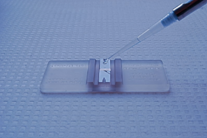
CC-BY-SA-2.0
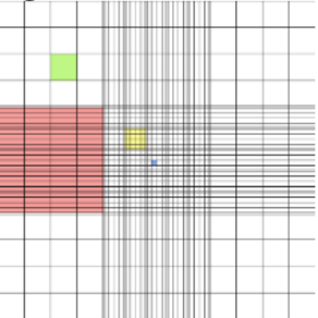
CC-BY-SA-3.0
Back in the day, I worked for a juice company in QC. One of the tests on OJ was to count fungal and insect contaminants via a Petroff-Hausser slide.
Prof. Kelly Burke
Electronic cell counters also count individual cells, typically as they flow past a laser (flow cytometry). Both of these methods count both live and dead cells and potentially any debris in the solution. You will not be performing a Direct Count in this lab.
The Standard Plate Count
Spread Plate Method of Isolation
In the SPC one wants to determine the density (number) of bacteria in a broth sample/specimen of bacteria of unknown density (number of cells/unit volume). One could take a small sample from the specimen, perhaps 1.0ml or 0.1ml and spread it across a petri dish to count the resulting colonies (remember that each colony is from one bacterial cell or unit). However, most specimens, based on the turbidity, might have millions of bacteria per ml in the sample. If 1.0ml was plated onto agar the number of bacteria would be so many that it would be impossible to count or even discern individual colonies. Therefore, one must perform a series of dilutions with the specimen to obtain a sample that will produce a plate on which colonies can be counted.
To do this, a known volume is taken from the original sample and placed in a dilution tube of a known volume, usually of sterile water or broth. After mixing, a known volume from the dilution tube is taken and placed in another dilution tube. This series of dilutions can be repeated a number of times resulting in progressively fewer cells in each tube down the line.

From the diluted mixtures one can then remove 1.0ml or 0.1ml and spread it over a plate of media. Somewhere in the series will be a “countable plate”. A countable plate is one that has between 30-300 CFU/ml (Colony Forming Units/ml). Fewer than 30 colonies (TFTC) and miscounts on a plate become statistically problematic. More than 300 colonies (TNTC) and counting becomes very difficult and errors are easily made! You’ll see this when you plate your samples.
Once one has counted the number of CFU on a plate, that number must be multiplied back by the amount the sample was diluted—the dilution factor. For example, if you dilute your sample by 100 times (meaning that the sample you used was 100x more dilute than the original specimen), you must multiply your count by 100 in order to determine the density of bacteria in the original specimen. There are several ways to calculate the dilutions in the series and the final dilutions plated. Any type of dilution can be made; however, in a SPC the dilutions are typically 1:10 or 1:100, which become fairly easy to calculate once you practice them and get the patterns. The process is illustrated in examples below.
Example \(\PageIndex{1}\)
A single dilution can be figured out by the following:
Amount transferred + volume of the dilution tube = DF (dilution factor)
If 1.0ml is transferred to a 9.0ml dilution tube then the dilution is:
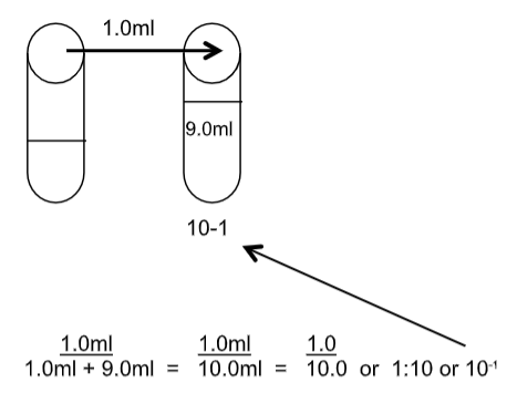
What would the dilution be if 0.1ml were added to 9.9ml? Show how you would determine this.
Solution
A series of dilutions is cumulative. Each tube is more dilute than the last, so the dilutions are compounded (multiplied together) as the series progresses:
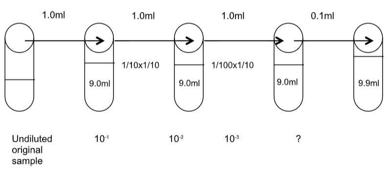
These dilutions can also be calculated with this commonly used equation:
\[V_1D_1 = V_2D_2 \nonumber \]
where V= volume; D= dilution
Let’s say you transferred 10.0ml from your original undiluted sample to a 90.0ml dilution tube. \(V_1\) is the volume you will transfer (10.0ml). \(D_1\) is always 1 because that is the starting dilution tube. \(V_2\) is the total volume in the next dilution tube once you’ve transferred your sample to it. So in this case,
\[\begin{align*}
10.0\mathit{ml} (1) &= 100.0\mathit{ml} (D_2); \text {solving for } D_2\\
10.0\mathit{ml}/100.0\mathit{ml}&= D_2\\
1/10&= D_2 \text { or}\\
10^{-1}& = D_2
\end{align*} \nonumber \]
Here is a more unusual example. Transfer 3.0ml into a dilution tube with 10.0ml (Why? Because one can! Not that one normally would…)
\[\begin{align*}
3.0\mathit{ml} (1) &= 10.0\mathit{ml} (D_2); \text {solving for } D_2\\
3.0\mathit{ml}/13.0\mathit{ml}&= D_2\\
0.23&= D_2 \text { or}\\
2.3\times 10^{-1}& = D_2
\end{align*} \nonumber \]
The next step is to plate your sample. Again, typically you would plate 1.0ml or 0.1ml depending on what you might need for your final dilutions. Show the Dilution Factor (DF) for each plate (the final dilution value for the plate):
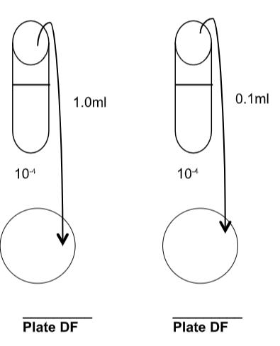
To determine the number (original cell density) of bacteria in the original sample:
Number of CFU:
OCD= Amount plated x dilution factor
If you diluted a plate 100x (1:100, or \(10^{-2}\)), transferred 1.0ml to an agar plate resulting in 65 colonies on the plate:
65 is the number of CFU
1.0 ml is the amount plated
\(10^{-2}\) is the dilution factor
So,
65 CFU
\(1.0\mathit{ml}l x 10^{-2} = 65 x 10^2 \text{CFU}/\mathit{ml} = 6.5 x 10^3 \text{CFU}/\mathit{ml} =\) the density of bacteria in your original specimen.
Contributors and Attributions
Kelly C. Burke (College of the Canyons)


