Biology LibreTexts

Section 11.5: Calculating Probabilities

  • Page ID
    27258
  • \( \newcommand{\vecs}[1]{\overset { \scriptstyle \rightharpoonup} {\mathbf{#1}} } \)

    \( \newcommand{\vecd}[1]{\overset{-\!-\!\rightharpoonup}{\vphantom{a}\smash {#1}}} \)

    \( \newcommand{\id}{\mathrm{id}}\) \( \newcommand{\Span}{\mathrm{span}}\)

    ( \newcommand{\kernel}{\mathrm{null}\,}\) \( \newcommand{\range}{\mathrm{range}\,}\)

    \( \newcommand{\RealPart}{\mathrm{Re}}\) \( \newcommand{\ImaginaryPart}{\mathrm{Im}}\)

    \( \newcommand{\Argument}{\mathrm{Arg}}\) \( \newcommand{\norm}[1]{\| #1 \|}\)

    \( \newcommand{\inner}[2]{\langle #1, #2 \rangle}\)

    \( \newcommand{\Span}{\mathrm{span}}\)

    \( \newcommand{\id}{\mathrm{id}}\)

    \( \newcommand{\Span}{\mathrm{span}}\)

    \( \newcommand{\kernel}{\mathrm{null}\,}\)

    \( \newcommand{\range}{\mathrm{range}\,}\)

    \( \newcommand{\RealPart}{\mathrm{Re}}\)

    \( \newcommand{\ImaginaryPart}{\mathrm{Im}}\)

    \( \newcommand{\Argument}{\mathrm{Arg}}\)

    \( \newcommand{\norm}[1]{\| #1 \|}\)

    \( \newcommand{\inner}[2]{\langle #1, #2 \rangle}\)

    \( \newcommand{\Span}{\mathrm{span}}\) \( \newcommand{\AA}{\unicode[.8,0]{x212B}}\)

    \( \newcommand{\vectorA}[1]{\vec{#1}}      % arrow\)

    \( \newcommand{\vectorAt}[1]{\vec{\text{#1}}}      % arrow\)

    \( \newcommand{\vectorB}[1]{\overset { \scriptstyle \rightharpoonup} {\mathbf{#1}} } \)

    \( \newcommand{\vectorC}[1]{\textbf{#1}} \)

    \( \newcommand{\vectorD}[1]{\overrightarrow{#1}} \)

    \( \newcommand{\vectorDt}[1]{\overrightarrow{\text{#1}}} \)

    \( \newcommand{\vectE}[1]{\overset{-\!-\!\rightharpoonup}{\vphantom{a}\smash{\mathbf {#1}}}} \)

    \( \newcommand{\vecs}[1]{\overset { \scriptstyle \rightharpoonup} {\mathbf{#1}} } \)

    \( \newcommand{\vecd}[1]{\overset{-\!-\!\rightharpoonup}{\vphantom{a}\smash {#1}}} \)

    \(\newcommand{\avec}{\mathbf a}\) \(\newcommand{\bvec}{\mathbf b}\) \(\newcommand{\cvec}{\mathbf c}\) \(\newcommand{\dvec}{\mathbf d}\) \(\newcommand{\dtil}{\widetilde{\mathbf d}}\) \(\newcommand{\evec}{\mathbf e}\) \(\newcommand{\fvec}{\mathbf f}\) \(\newcommand{\nvec}{\mathbf n}\) \(\newcommand{\pvec}{\mathbf p}\) \(\newcommand{\qvec}{\mathbf q}\) \(\newcommand{\svec}{\mathbf s}\) \(\newcommand{\tvec}{\mathbf t}\) \(\newcommand{\uvec}{\mathbf u}\) \(\newcommand{\vvec}{\mathbf v}\) \(\newcommand{\wvec}{\mathbf w}\) \(\newcommand{\xvec}{\mathbf x}\) \(\newcommand{\yvec}{\mathbf y}\) \(\newcommand{\zvec}{\mathbf z}\) \(\newcommand{\rvec}{\mathbf r}\) \(\newcommand{\mvec}{\mathbf m}\) \(\newcommand{\zerovec}{\mathbf 0}\) \(\newcommand{\onevec}{\mathbf 1}\) \(\newcommand{\real}{\mathbb R}\) \(\newcommand{\twovec}[2]{\left[\begin{array}{r}#1 \\ #2 \end{array}\right]}\) \(\newcommand{\ctwovec}[2]{\left[\begin{array}{c}#1 \\ #2 \end{array}\right]}\) \(\newcommand{\threevec}[3]{\left[\begin{array}{r}#1 \\ #2 \\ #3 \end{array}\right]}\) \(\newcommand{\cthreevec}[3]{\left[\begin{array}{c}#1 \\ #2 \\ #3 \end{array}\right]}\) \(\newcommand{\fourvec}[4]{\left[\begin{array}{r}#1 \\ #2 \\ #3 \\ #4 \end{array}\right]}\) \(\newcommand{\cfourvec}[4]{\left[\begin{array}{c}#1 \\ #2 \\ #3 \\ #4 \end{array}\right]}\) \(\newcommand{\fivevec}[5]{\left[\begin{array}{r}#1 \\ #2 \\ #3 \\ #4 \\ #5 \\ \end{array}\right]}\) \(\newcommand{\cfivevec}[5]{\left[\begin{array}{c}#1 \\ #2 \\ #3 \\ #4 \\ #5 \\ \end{array}\right]}\) \(\newcommand{\mattwo}[4]{\left[\begin{array}{rr}#1 \amp #2 \\ #3 \amp #4 \\ \end{array}\right]}\) \(\newcommand{\laspan}[1]{\text{Span}\{#1\}}\) \(\newcommand{\bcal}{\cal B}\) \(\newcommand{\ccal}{\cal C}\) \(\newcommand{\scal}{\cal S}\) \(\newcommand{\wcal}{\cal W}\) \(\newcommand{\ecal}{\cal E}\) \(\newcommand{\coords}[2]{\left\{#1\right\}_{#2}}\) \(\newcommand{\gray}[1]{\color{gray}{#1}}\) \(\newcommand{\lgray}[1]{\color{lightgray}{#1}}\) \(\newcommand{\rank}{\operatorname{rank}}\) \(\newcommand{\row}{\text{Row}}\) \(\newcommand{\col}{\text{Col}}\) \(\renewcommand{\row}{\text{Row}}\) \(\newcommand{\nul}{\text{Nul}}\) \(\newcommand{\var}{\text{Var}}\) \(\newcommand{\corr}{\text{corr}}\) \(\newcommand{\len}[1]{\left|#1\right|}\) \(\newcommand{\bbar}{\overline{\bvec}}\) \(\newcommand{\bhat}{\widehat{\bvec}}\) \(\newcommand{\bperp}{\bvec^\perp}\) \(\newcommand{\xhat}{\widehat{\xvec}}\) \(\newcommand{\vhat}{\widehat{\vvec}}\) \(\newcommand{\uhat}{\widehat{\uvec}}\) \(\newcommand{\what}{\widehat{\wvec}}\) \(\newcommand{\Sighat}{\widehat{\Sigma}}\) \(\newcommand{\lt}{<}\) \(\newcommand{\gt}{>}\) \(\newcommand{\amp}{&}\) \(\definecolor{fillinmathshade}{gray}{0.9}\)

    Once the mode of inheritance of a disease or trait is identified, some inferences about the genotype of individuals in a pedigree can be made, based on their phenotypes and where they appear in the family tree. Given these genotypes, it is possible to calculate the probability of a particular genotype being inherited in subsequent generations. This can be useful in genetic counseling, for example when prospective parents wish to know the likelihood of their offspring inheriting a disease for which they have a family history.

    Probabilities in pedigrees are calculated using knowledge of Mendelian inheritance and the same basic methods as are used in other fields. The first formula is the product rule: the joint probability of two independent events is the product of their individual probabilities; this is the probability of one event AND another event occurring. For example, the probability of a rolling a “five” with a single throw of a single six-sided die is 1/6, and the probability of rolling “five” in each of three successive rolls is 1/6 x 1/6 x 1/6 = 1/216. The second useful formula is the sum rule, which states that the combined probability of two independent events is the sum of their individual probabilities. This is the probability of one event OR another event occurring. For example, the probability of rolling a five or six in a single throw of a dice is 1/6 + 1/6 = 1/3.

    With these rules in mind, we can calculate the probability that two carriers (i.e. heterozygotes) of an AR disease will have a child affected with the disease as ½ x ½ = ¼, since for each parent, the probability of any gametes carrying the disease allele is ½. This is consistent with what we already know from calculating probabilities using a Punnett Square (e.g. in a monohybrid cross Aa x Aa, ¼ of the offspring are aa).

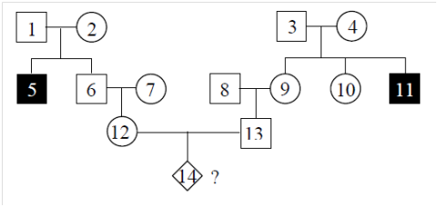
    We can likewise calculate probabilities in the more complex pedigree shown in Figure \(\PageIndex{11}\).

    Fig5.11.png
    Figure \(\PageIndex{11}\): Individuals in this pedigree are labeled with numbers to make discussion easier. (Original-Deyholos-CC:AN)

    Assuming the disease has an AR pattern of inheritance, what is the probability that individual 14 will be affected? We can assume that individuals #1, #2, #3 and #4 are heterozygotes (Aa), because they each had at least one affected (aa) child, but they are not affected themselves. This means that there is a 2/3 chance that individual #6 is also Aa. This is because according to Mendelian inheritance, when two heterozygotes mate, there is a 1:2:1 distribution of genotypes AA:Aa:aa. However, because #6 is unaffected, he can’t be aa, so he is either Aa or AA, but the probability of him being Aa is twice as likely as AA. By the same reasoning, there is likewise a 2/3 chance that #9 is a heterozygous carrier of the disease allele.

    If individual 6 is a heterozygous for the disease allele, then there is a ½ chance that #12 will also be a heterozygote (i.e. if the mating of #6 and #7 is Aa × AA, half of the progeny will be Aa; we are also assuming that #7, who is unrelated, does not carry any disease alleles). Therefore, the combined probability that #12 is also a heterozygote is 2/3 x 1/2 = 1/3. This reasoning also applies to individual #13, i.e. there is a 1/3 probability that he is a heterozygote for the disease. Thus, the overall probability that both individual #12 and #13 are heterozygous, and that a particular offspring of theirs will be homozygous for the disease alleles is 1/3 x 1/3 x 1/4 = 1/36.


    This page titled Section 11.5: Calculating Probabilities is shared under a CC BY-SA 3.0 license and was authored, remixed, and/or curated by Todd Nickle and Isabelle Barrette-Ng via source content that was edited to the style and standards of the LibreTexts platform.