Biology LibreTexts

Section 7.7: Mapping With Three-Point Crosses

  • Page ID
    27275
  • \( \newcommand{\vecs}[1]{\overset { \scriptstyle \rightharpoonup} {\mathbf{#1}} } \)

    \( \newcommand{\vecd}[1]{\overset{-\!-\!\rightharpoonup}{\vphantom{a}\smash {#1}}} \)

    \( \newcommand{\id}{\mathrm{id}}\) \( \newcommand{\Span}{\mathrm{span}}\)

    ( \newcommand{\kernel}{\mathrm{null}\,}\) \( \newcommand{\range}{\mathrm{range}\,}\)

    \( \newcommand{\RealPart}{\mathrm{Re}}\) \( \newcommand{\ImaginaryPart}{\mathrm{Im}}\)

    \( \newcommand{\Argument}{\mathrm{Arg}}\) \( \newcommand{\norm}[1]{\| #1 \|}\)

    \( \newcommand{\inner}[2]{\langle #1, #2 \rangle}\)

    \( \newcommand{\Span}{\mathrm{span}}\)

    \( \newcommand{\id}{\mathrm{id}}\)

    \( \newcommand{\Span}{\mathrm{span}}\)

    \( \newcommand{\kernel}{\mathrm{null}\,}\)

    \( \newcommand{\range}{\mathrm{range}\,}\)

    \( \newcommand{\RealPart}{\mathrm{Re}}\)

    \( \newcommand{\ImaginaryPart}{\mathrm{Im}}\)

    \( \newcommand{\Argument}{\mathrm{Arg}}\)

    \( \newcommand{\norm}[1]{\| #1 \|}\)

    \( \newcommand{\inner}[2]{\langle #1, #2 \rangle}\)

    \( \newcommand{\Span}{\mathrm{span}}\) \( \newcommand{\AA}{\unicode[.8,0]{x212B}}\)

    \( \newcommand{\vectorA}[1]{\vec{#1}}      % arrow\)

    \( \newcommand{\vectorAt}[1]{\vec{\text{#1}}}      % arrow\)

    \( \newcommand{\vectorB}[1]{\overset { \scriptstyle \rightharpoonup} {\mathbf{#1}} } \)

    \( \newcommand{\vectorC}[1]{\textbf{#1}} \)

    \( \newcommand{\vectorD}[1]{\overrightarrow{#1}} \)

    \( \newcommand{\vectorDt}[1]{\overrightarrow{\text{#1}}} \)

    \( \newcommand{\vectE}[1]{\overset{-\!-\!\rightharpoonup}{\vphantom{a}\smash{\mathbf {#1}}}} \)

    \( \newcommand{\vecs}[1]{\overset { \scriptstyle \rightharpoonup} {\mathbf{#1}} } \)

    \( \newcommand{\vecd}[1]{\overset{-\!-\!\rightharpoonup}{\vphantom{a}\smash {#1}}} \)

    \(\newcommand{\avec}{\mathbf a}\) \(\newcommand{\bvec}{\mathbf b}\) \(\newcommand{\cvec}{\mathbf c}\) \(\newcommand{\dvec}{\mathbf d}\) \(\newcommand{\dtil}{\widetilde{\mathbf d}}\) \(\newcommand{\evec}{\mathbf e}\) \(\newcommand{\fvec}{\mathbf f}\) \(\newcommand{\nvec}{\mathbf n}\) \(\newcommand{\pvec}{\mathbf p}\) \(\newcommand{\qvec}{\mathbf q}\) \(\newcommand{\svec}{\mathbf s}\) \(\newcommand{\tvec}{\mathbf t}\) \(\newcommand{\uvec}{\mathbf u}\) \(\newcommand{\vvec}{\mathbf v}\) \(\newcommand{\wvec}{\mathbf w}\) \(\newcommand{\xvec}{\mathbf x}\) \(\newcommand{\yvec}{\mathbf y}\) \(\newcommand{\zvec}{\mathbf z}\) \(\newcommand{\rvec}{\mathbf r}\) \(\newcommand{\mvec}{\mathbf m}\) \(\newcommand{\zerovec}{\mathbf 0}\) \(\newcommand{\onevec}{\mathbf 1}\) \(\newcommand{\real}{\mathbb R}\) \(\newcommand{\twovec}[2]{\left[\begin{array}{r}#1 \\ #2 \end{array}\right]}\) \(\newcommand{\ctwovec}[2]{\left[\begin{array}{c}#1 \\ #2 \end{array}\right]}\) \(\newcommand{\threevec}[3]{\left[\begin{array}{r}#1 \\ #2 \\ #3 \end{array}\right]}\) \(\newcommand{\cthreevec}[3]{\left[\begin{array}{c}#1 \\ #2 \\ #3 \end{array}\right]}\) \(\newcommand{\fourvec}[4]{\left[\begin{array}{r}#1 \\ #2 \\ #3 \\ #4 \end{array}\right]}\) \(\newcommand{\cfourvec}[4]{\left[\begin{array}{c}#1 \\ #2 \\ #3 \\ #4 \end{array}\right]}\) \(\newcommand{\fivevec}[5]{\left[\begin{array}{r}#1 \\ #2 \\ #3 \\ #4 \\ #5 \\ \end{array}\right]}\) \(\newcommand{\cfivevec}[5]{\left[\begin{array}{c}#1 \\ #2 \\ #3 \\ #4 \\ #5 \\ \end{array}\right]}\) \(\newcommand{\mattwo}[4]{\left[\begin{array}{rr}#1 \amp #2 \\ #3 \amp #4 \\ \end{array}\right]}\) \(\newcommand{\laspan}[1]{\text{Span}\{#1\}}\) \(\newcommand{\bcal}{\cal B}\) \(\newcommand{\ccal}{\cal C}\) \(\newcommand{\scal}{\cal S}\) \(\newcommand{\wcal}{\cal W}\) \(\newcommand{\ecal}{\cal E}\) \(\newcommand{\coords}[2]{\left\{#1\right\}_{#2}}\) \(\newcommand{\gray}[1]{\color{gray}{#1}}\) \(\newcommand{\lgray}[1]{\color{lightgray}{#1}}\) \(\newcommand{\rank}{\operatorname{rank}}\) \(\newcommand{\row}{\text{Row}}\) \(\newcommand{\col}{\text{Col}}\) \(\renewcommand{\row}{\text{Row}}\) \(\newcommand{\nul}{\text{Nul}}\) \(\newcommand{\var}{\text{Var}}\) \(\newcommand{\corr}{\text{corr}}\) \(\newcommand{\len}[1]{\left|#1\right|}\) \(\newcommand{\bbar}{\overline{\bvec}}\) \(\newcommand{\bhat}{\widehat{\bvec}}\) \(\newcommand{\bperp}{\bvec^\perp}\) \(\newcommand{\xhat}{\widehat{\xvec}}\) \(\newcommand{\vhat}{\widehat{\vvec}}\) \(\newcommand{\uhat}{\widehat{\uvec}}\) \(\newcommand{\what}{\widehat{\wvec}}\) \(\newcommand{\Sighat}{\widehat{\Sigma}}\) \(\newcommand{\lt}{<}\) \(\newcommand{\gt}{>}\) \(\newcommand{\amp}{&}\) \(\definecolor{fillinmathshade}{gray}{0.9}\)

    A particularly efficient method of mapping three genes at once is the three-point cross, which allows the order and distance between three potentially linked genes to be determined in a single cross experiment (Figure \(\PageIndex{12}\)). This is particularly useful when mapping a new mutation with an unknown location to two previously mapped loci. The basic strategy is the same as for the dihybrid mapping experiment; pure breeding lines with contrasting genotypes are crossed to produce an individual heterozygous at three loci (a trihybrid), which is then testcrossed to determine the recombination frequency between each pair of genes.
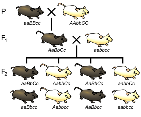
    Fig7.12.png
    Figure \(\PageIndex{12}\): A three point cross for loci affecting tail length, fur color, and whisker length. (Original-Modified Deyholos-CC:AN)

    One useful feature of the three-point cross is that the order of the loci relative to each other can usually be determined by a simple visual inspection of the F2 segregation data. If the genes are linked, there will often be two phenotypic classes that are much more infrequent than any of the others. In these cases, the rare phenotypic classes are usually those that arose from two crossover events, in which the locus in the middle is flanked by a crossover on either side of it. Thus, among the two rarest recombinant phenotypic classes, the one allele that differs from the other two alleles relative to the parental genotypes likely represents the locus that is in the middle of the other two loci. For example, based on the phenotypes of the pure-breeding parents in Figure \(\PageIndex{12}\), the parental genotypes are aBC and AbC (remember the order of the loci is unknown, and it is not necessarily the alphabetical order in which we wrote the genotypes). Because we can deduce from the outcome of the testcross (Table \(\PageIndex{2}\)) that the rarest genotypes were abC and ABc, we can conclude that locus A that is most likely located between the other two loci, since it would require a recombination event between both A and B and between A and C in order to generate these gametes. Thus, the order of loci is BAC (which is equivalent to CAB).

    Table \(\PageIndex{2}\): An example of data that might be obtained from the F2 generation of the three-point cross shown in Figure \(\PageIndex{12}\). The rarest phenotypic classes correspond to double recombinant gametes ABc and abC. Each phenotypic class and the gamete from the trihybrid that produced it can also be classified as parental (P) or recombinant (R) with respect to each pair of loci (A,B), (A,C), (B,C) analyzed in the experiment.

    tail phenotype

    fur phenotype

    whisker phenotype

    number of progeny

    gamete from trihybrid

    genotype of F2 from test cross

    loci A, B

    loci A, C

    loci B, C

    short

    brown

    long

    5

    aBC

    aaBbCc

    P

    R

    R

    long

    white

    long

    38

    AbC

    AabbCc

    P

    P

    P

    short

    white

    long

    1

    abC

    aabbCc

    R

    R

    P

    long

    brown

    long

    16

    ABC

    AaBbCc

    R

    P

    R

    short

    brown

    short

    42

    aBc

    aaBbcc

    P

    P

    P

    long

    white

    short

    5

    Abc

    Aabbcc

    P

    R

    R

    short

    white

    short

    12

    abc

    aabbcc

    R

    P

    R

    long

    brown

    short

    1

    ABc

    AaBbcc

    R

    R

    P

    Recombination frequencies may be calculated for each pair of loci in the three-point cross as we did before for one pair of loci in our dihybrid (Figure 7. 8).

    \[\begin{alignat}{2} \textrm{loci A,B R.F.} = &\dfrac{1+16+12+1}{120} &&= 25\%\\ \textrm{loci A,C R.F.} = &\dfrac{1+5+1+5}{120} &&= 10\%\\ \textrm{loci B,C R.F.} = &\dfrac{5+16+12+5}{120} &&= 32\%\\ \textrm{(not corrected for double}\\ \textrm{crossovers)}\hspace{40px} \end{alignat}\]

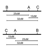
    However, note that in the three point cross, the sum of the distances between A-B and A-C (35%) is less than the distance calculated for B-C (32%)(Figure \(\PageIndex{13}\)). this is because of double crossovers between B and C, which were undetected when we considered only pairwise data for B and C. We can easily account for some of these double crossovers, and include them in calculating the map distance between B and C, as follows. We already deduced that the map order must be BAC (or CAB), based on the genotypes of the two rarest phenotypic classes in Table \(\PageIndex{2}\). However, these double recombinants, ABc and abC, were not included in our calculations of recombination frequency between loci B and C. If we included these double recombinant classes (multiplied by 2, since they each represent two recombination events), the calculation of recombination frequency between B and C is as follows, and the result is now more consistent with the sum of map distances between A-B and A-C.

    \[\begin{align} \textrm{loci B,C R.F.} &= \dfrac{5+16+12+5+2(1)+2(1)}{120} = 35\%\\ \textrm{(corrected for double}&\\ \textrm{recombinants)}& \end{align}\]

    Fig7.13.png
    Figure \(\PageIndex{13}\): Equivalent maps based on the data in Table \(\PageIndex{2}\) (without correction for double crossovers). (Original-Deyholos-CC:AN)

    Thus, the three point cross was useful for:

    1. determining the order of three loci relative to each other,
    2. calculating map distances between the loci, and
    3. detecting some of the double crossover events that would otherwise lead to an underestimation of map distance.

    However, it is possible that other, double crossovers events remain undetected, for example double crossovers between loci A,B or between loci A,C. Geneticists have developed a variety of mathematical procedures to try to correct for things like double crossovers during large-scale mapping experiments.

    As more and more genes are mapped a better genetic map can be constructed. Then, when a new gene is discovered, it can be mapped relative to other genes of known location to determine its location. All that is needed to map a gene is two alleles, a wild type allele (e.g. A) and a mutant allele (e.g. 'a').


    This page titled Section 7.7: Mapping With Three-Point Crosses is shared under a CC BY-SA 3.0 license and was authored, remixed, and/or curated by Todd Nickle and Isabelle Barrette-Ng via source content that was edited to the style and standards of the LibreTexts platform.