20.1: Epidemiology

A statistical correlation between two phenomena is simply that. It does not prove that one phenomenon caused the other. Just because A is often associated with B, does not prove that A causes B. Example: the incidence of cirrhosis of the liver is associated with cigarette smoking. Does smoking cause cirrhosis? Probably not. Excessive consumption of alcohol is a more likely cause. However, as heavy drinkers tend to be heavy smokers, the statistical association is there, but in this case is probably a confounding variable. How can one establish that A causes B? In the laboratory you could set up a controlled experiment treating one group of animals with A and having a second control group without A but otherwise treated the same (thus avoiding confounding variables). Such experimentation is rarely possible (or ethical) in humans so we must turn to the methods and criteria of epidemiology.

John Snow - the First Epidemiologist

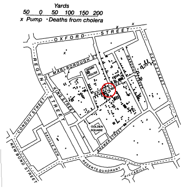
During an outbreak of cholera in London in 1854, John Snow plotted on a map the location of all the cases he learned of. Water in that part of London was pumped from wells located in the various neighborhoods. Snow's map revealed a close association between the density of cholera cases and a single well located on Broad Street. The Broad Street well is marked with an X (within the red circle) in the above figure. Removing the pump handle of the Broad Street well put an end to the epidemic. This despite the fact that the infectious agent that causes cholera was not clearly recognized until 1905.

Figure \(\PageIndex{1}\): John Snow's map showing cholera deaths in London in 1854 (courtesy of The Geographical Journal)

Although an association between two phenomena is no more than that, one can apply several criteria to gauge the strength of the association, and if it is strong, infer that one phenomenon causes the other.

The five criteria to gauge the strength of the association

• a high relative risk
• consistency
• a graded response to a graded dose
• a temporal relationship
• a plausible mechanism

Cigarette Smoking: A Case Study

In Table \(\PageIndex{1}\), the quotient of observed deaths divided by expected deaths (those in the control group) gives the relative death rate. This value is a measure of risk. Although smoking is associated with many more cases of heart disease than of lung cancer, lung cancer is the disease with the highest relative risk for smokers. The relative death rate from lung cancer is over 10 times greater in smokers than in non-smokers. This is strong evidence that smoking causes lung cancer. Cigarette smoking is estimated to be directly responsible for 80–90% of all lung cancer deaths (which totalled 160,390 in the U.S. in 2007).

This table gives the number of deaths from various causes in a prospective study of cigarette smokers ("observed deaths") compared with the number to be expected among nonsmokers of the same ages ("expected deaths"). The differences between the two represent "excess deaths". The contribution of each disease to the total of excess deaths is given as the "percentage of excess". Note that coronary artery disease accounts for one half of the excess deaths in the smoking group.

Table \(\PageIndex{1}\): Observed deaths, expected deaths, and relative death rates.

Cause of Death	Observed Deaths	Expected Deaths	Excess Deaths	Percentage of Excess	Relative Death Rate
Total deaths (all causes)	7316	4651	2665	100.0	1.57
Coronary artery disease	3361	1973	1388	52.1	1.70
Other heart disease	503	425	78	2.9	1.18
Cerebrovascular lesions	556	428	128	4.8	1.30
Aneurysm & Buerger's disease	86	29	57	2.1	2.97
Other circulatory diseases	87	68	19	0.7	1.28
Lung cancer	397	37	360	13.5	10.73
Cancer of mouth, larynx, or esophagus	91	18	73	2.7	5.06
Cancer of the bladder	70	35	35	1.3	2.00
Other cancers	902	651	251	9.4	1.39
Gastric & duodenal ulcer	100	25	75	2.8	4.00
Cirrhosis of the liver	83	43	40	1.5	1.93
Pulmonary disease (except cancer)	231	81	150	5.6	2.85
All other diseases	486	453	33	1.2	1.07
Accident, violence, suicide	363	385	-22	-0.8	0.94

Dividing the number of observed deaths by the number of expected deaths gives the "relative death rate" for each disease. This shows that smokers die of lung cancer 10 times as often (10.73, above) as do nonsmokers, which is a very high relative risk. However, in both groups lung cancer is rarer than coronary artery disease. (Data from E. C. Hammond and D. Dorn, 1966.)

Consistency

Our confidence that A causes B is strengthened when different studies using different populations all show the same association. The earliest studies of smoking were retrospective; that is, after a disease was diagnosed, the patient's smoking habits were determined. Later studies were prospective. A prospective study selects a population in good health and meeting any other desired criteria (smoking habits in this case) and follows it over a period of years to see what happens to its members.

Figure \(\PageIndex{2}\): Relationship between smoking and death

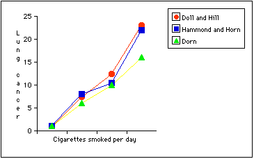
This graph shows essentially the same relationship between smoking and deaths from lung cancer in three different groups (totalling over a million people) studied prospectively. Doll and Hill studied a group of British physicians. Dorn followed the health of a group of U.S. veterans. Horn studied 187,783 U.S. male volunteers. In each case the relative death rates are graphed as a function of number of cigarettes smoked each day (from zero at the left to over a pack at the right).

A Graded Response to a Graded Dose

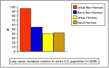
All three studies graphed above show that the relative death rate from lung cancer increased with an increase in the average number of cigarettes smoked each day. One goal of picking different groups to study is to avoid confounding variables. If, for example, all the groups studied lived in cities, it would be difficult to distinguish between the effects of smoking and the effects of general air pollution.

Figure \(\PageIndex{3}\): Utah smokers

This graph compares the incidence of lung cancer among male Mormons and non-Mormons living in urban and rural areas of Utah. Male non-Mormons living in the city have a higher risk of developing lung cancer than those living in the country. Is this because of smoking or because of the pollution of urban air? It appears to be the former because Mormons show no such city vs. country difference, and cigarette smoking is prohibited for Mormons. Studies like these help to eliminate the effect of confounding variables. Probably less than 5% of lung cancer is caused by breathing polluted city air.

Temporal Relationship

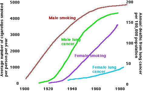
If A causes B, then exposure to A must have preceded the onset of B. Establishing cause-effect relationships for possible carcinogens has been particularly difficult because for cancers, the latency period between exposure and illness is often many years. Nonetheless, data such as those shown in this graph, provide another strong link in the case against cigarettes.

Figure \(\PageIndex{4}\): Cause - effect relationship for possible carcinogens

In recent decades, sales of cigarettes in the U.S. have dropped, both on a per capita basis and in absolute numbers. Whereas half of adult males smoked in the mid-sixties, less than a third do today. This change has already caused the rate of lung cancer in males to level off. Unfortunately, the rate is still rising for women (and in 1987 surpassed breast cancer as the leading cause of cancer deaths in U.S. women).

Plausible Mechanism

Over 40 different chemicals found in cigarette smoke cause an increase in cancer when given over several years to laboratory rats.

So how strong is the case against cigarettes?

Defenders of the tobacco industry frequently claim that no one has proved that cigarette smoking causes lung cancer. In one sense they are right. Proof from epidemiology differs from proof in a laboratory experiment. What we have seen here is that the more closely we can meet the several criteria linking A and B, the more confident we can be that A causes B.

Few epidemiological studies have met these criteria better than those studying the statistical relationship between smoking and health. Smoking is probably the greatest single cause of preventable illness in the United States.

Rules to live by

Hardly a week goes by these days without a report in the press and on TV of another link between an environmental agent and human disease. Does living near nuclear power stations increase one's risk of cancer? living near electric power lines? Does a diet rich in saturated fats predispose U.S. males (but, for some reason, not French males) to early death from coronary artery disease?

I hope that your ability to interpret the avalanche of reported associations - and any adjustments that you make in your life as a result - will benefit from your applying to such reports the five criteria outlined here.