6.3: Kinetics with Enzymes

Search Fundamentals of Biochemistry

Learning Goals 

(Learning goals written by Claude, Sonnet 4.6, Anthropic)

Deriving the Michaelis-Menten Equation: Two Approaches

• Follow the derivation of the Michaelis-Menten equation v₀ = V_M[S]/(K_M + [S]) under the rapid equilibrium assumption — in which k₂ >> k₃ so that K_M = K_S = k₂/k₁ is the true dissociation constant for ES — using mass balance for E (E₀ = [E] + [ES]) and the expression v₀ = k₃[ES], and explain why K_M equals K_S only under this limiting condition.
• Follow the derivation of the Michaelis-Menten equation under the steady state assumption — in which d[ES]/dt ≈ 0 but k₂ is not necessarily >> k₃ — showing that K_M = (k₂ + k₃)/k₁ and explaining why K_M in this general case is not the thermodynamic dissociation constant for ES but rather an operational constant that approaches K_S only when k₂ >> k₃.
• Extend the Michaelis-Menten framework to an enzyme mechanism with a covalent intermediate (E + S ↔ ES → E-P + Q, then E-P + H₂O → E + P) — showing that the same hyperbolic equation results but with k_cat = k₂k₃/(k₂ + k₃) — and explain the "burst phase" kinetics observed for product Q when k₂ >> k₃, distinguishing it from the subsequent steady-state phase used to determine true VM.

Interpreting Kinetic Parameters

• Define and physically interpret the three key kinetic parameters — K_M (substrate concentration at half-maximal velocity, in units of M; an effective but not necessarily thermodynamic K_D), k_cat (turnover number in s⁻¹, the number of substrate molecules converted to product per active site per second at saturating S), and k_cat/K_M (the second-order specificity constant in M⁻¹s⁻¹ that governs reaction rate when S << KM and that approaches the diffusion limit of ~10⁸–10⁹ M⁻¹s⁻¹ for the fastest enzymes) — and explain how k_cat/K_M is used to compare an enzyme's efficiency with competing substrates.
• Describe the limiting behaviors of the Michaelis-Menten equation: when [S] << K_M, v₀ = (k_cat/K_M)[E₀][S] (second-order kinetics, rate depends linearly on both S and E₀); when [S] >> K_M, v₀ = V_M = kcat[E₀] (zero-order in S, first-order in E₀); and when [S] = K_M, v₀ = V_M/2 — and explain why enzyme-catalyzed reactions appear to saturate while uncatalyzed first-order reactions do not.

Experimental Determination and Graphical Analysis

• Explain why initial velocities v₀ are used rather than velocities at later time points in Michaelis-Menten analysis, describe how v₀ is determined from the initial slope of a P vs. t progress curve when [S] ≈ S₀, and compare the information content and practical tradeoffs of the Michaelis-Menten hyperbolic plot, the Lineweaver-Burk double-reciprocal plot (slope = K_M/V_M, y-intercept = 1/V_M, x-intercept = −1/K_M), the Scatchard plot, and the Eadie-Hofstee plot (v₀ vs. v₀/[S], slope = −K_M, y-intercept = V_M) — explaining why nonlinear fitting to the hyperbola is statistically preferred over linear transformation methods.
• Describe how the reversible Michaelis-Menten equation — which includes terms for both forward and reverse reactions with K_MS, K_MP, k_cat(forward), and k_cat(reverse) — extends the irreversible equation to account for product-to-substrate conversion, and explain why the net forward velocity equation is not simply the difference of the two unidirectional rate equations but requires a unified derivation that accounts for both directions simultaneously.

 

An enzyme alters the pathway for converting a reactant to a product by binding to the reactant, facilitating the intramolecular conversion of the bound substrate to the bound product, and then releasing the product. Enzymes do not affect the thermodynamics of reactions. For reversible reactions (as an example), the equilibrium constant, K_eq, is unchanged. What is charged is the rate at which equilibrium is achieved. Enzymes lower the activation energy for bound transition states and change the reaction mechanism.

Figure \(\PageIndex{1}\) shows the simplest chemical reaction that can be written to show how an enzyme catalyzes a reaction.

Figure \(\PageIndex{1}\): Chemical equation for a simple enzyme-catalyzed reaction

Rapid Equilibrium Enzyme-Catalyzed Reactions

We have previously derived equations for the reversible binding of a ligand to a macromolecule. Next, we derived equations for the receptor-mediated facilitated transport of a molecule through a semipermeable membrane. This latter case extended the former case by adding a physical transport step. Now, in what hopefully will seem like deja vu, we will derive almost identical equations for the chemical transformation of a ligand, commonly referred to as a substrate, into a product by an enzyme. We will study two scenarios based on two different assumptions, each enabling a straightforward mathematical derivation of kinetic equations:

1. Rapid Equilibrium Assumption - enzyme E (macromolecule) and substrate S (ligand) concentrations can be determined using the dissociation constant since E, S, and ES are in rapid equilibrium, as we previously used in deriving the equations for facilitated transport. Sorry about the switch from A to S in the substrate designation. Biochemists use S to represent the substrate (ligand), and A, B, P, and Q to represent reactants and products in multi-substrate, multi-product reactions.
2. Steady State Assumption (more general) - enzyme and substrate concentrations are not those determined using the dissociation constant.

Enzyme kinetics experiments, as we will see in the following chapters, must be used to determine the detailed mechanism of the catalyzed reaction. Using kinetic analysis, you can determine the order in which substrates and products bind and dissociate, the rate constants for individual steps, and clues to the mechanism used by the enzyme in catalysis.

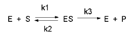
Consider the following reaction mechanism for the enzyme-catalyzed conversion of substrate S into product P. (We will assume that the catalyzed rate is much greater than the noncatalyzed rate.)

\[\ce{E +S <=>[K_s] ES ->[k_3] E + P} \nonumber \]

As we did for the derivation of the equations for the facilitated transport reactions under rapid equilibrium conditions, this derivation is based on the assumption that the relative concentrations of S, E, and ES can be determined by the dissociation constant, K_S, for the interactions and the concentrations of each species during the early part of the reaction (i.e., under initial rate conditions). Assume also the S >> E₀. Remember that under these conditions, S changes little over time. Is this a valid assumption? Examine the mechanism shown above. S binds to E with a second-order rate constant k₁. ES has two fates. It can dissociate to S + E with a first-order rate constant k₂, or it can be converted to the product P + E with a first-order rate constant k₃. If we assume that k₂ >> k₃ (i.e., that the complex falls apart much more quickly than S is converted to P), then the relative ratios of S, E, and ES can be described by Ks. Alternatively, you can think about it this way. If S binds to E, most of S will dissociate, and a small amount will be converted to P. If it does, then E is now free and will quickly bind S and reequilibrate since the most likely fate of bound S is to dissociate, not be converted to P (since \(k_3 \ll k_2\)). This also makes sense if you consider that the physical step, characterized by k₂, is likely to be quicker than the chemical step, characterized by k₃. Hence, the following assumptions have been used:

• \(S \gg E_0\)
• \(P_0 = 0\)
• \(k_3\) is rate-limiting (i.e., the slow step)

We will derive equations relating the initial velocity v to the initial substrate concentration S₀, assuming that P is negligible over the time interval used to measure the initial velocity. Also assume that \(v_{catalyzed} \gg v_{noncatalyzed}\). In contrast to the first-order reaction of S to P in the absence of E, v is not proportional to S₀ but to S_bound. Therefore, \(v \propto [ES]\), or

\[v = {const} [ES] = k_3 [ES] \label{EQ10} \]

where \(v\) is the velocity (i.e., reaction rate).

Now, let's get \(ES\) from the dissociation constant K_S (assuming rapid equilibrium of E, S, and ES) and mass balance for E (E₀ = E + ES, so E = E₀ - ES). We will use mass balance for S when deriving the steady-state equation. In many cases, S is approximately equal to S₀ or the total amount of substrate. This makes sense if you consider that the enzyme is a catalyst that acts repeatedly to produce the product, so you don't need significant amounts of the enzyme. The resulting equation of [ES] is shown below.

\begin{equation}
(E S)=\frac{\left(E_0\right)(S)}{K_S+(S)}
\end{equation}

A derivation of [ES] under rapid equilibrium conditions

Here it is!

Derivation

\begin{equation}
\begin{gathered}
K_S=\frac{[E][S]}{[E S]}=\left(\frac{\left.\left(\left[E_0\right]-[E S]\right)[S]\right)}{[E S]}\right. \\
(E S) K_S=\left(E_0\right)(S)-(E S)(S) \\
(E S) K_S+(E S)(S)=\left(E_0\right)(S) \\
(E S)\left(K_S+(S)\right)=\left(E_0\right)(S)
\end{gathered}
\end{equation}

This derivation assumes that we know S (equal to S₀) and E_tot (which is E₀).

Let us assume that S is much greater than E, as is the likely biological case. We can calculate ES using the following equations and the same procedure we used for the derivation of the binding equation, which gives the equation below:

\begin{equation}
[E S]=\frac{\left[E_0\right][S]}{K_S+S}
\end{equation}

which is analogous to

\begin{equation}
[M L]=\frac{\left[M_0\right][S]}{K_D+L}
\end{equation}

This leads to

\begin{equation}
v_0=\frac{\left(k_3\right)\left(E_0\right)(S)}{K_S+(S)}=\frac{\left(V_M\right)(S)}{K_S+(S)}
\end{equation}

where

\begin{equation}
V_M=k_3 E_0
\end{equation}

This is the world-famous Henri-Michaelis-Menten Equation. It is a hyperbola just like the graph for the binding of a ligand to a macromolecule with a given dissociation constant, K_D^.

Move the sliders in the interactive graph below to see how changing Km and Vm alters the graph. Note that this graph is identical to the graph for M + L ↔ ML.

​

Just as in the case with noncatalyzed first-order decay, it is easiest to measure the initial velocity of the reaction when [S] does not change much with time, and the velocity is constant (i.e., the slope of the dP/dt curve is constant). A plot of [P] vs t (called a progress curve) is made for each studied substrate concentration. From these curves, the initial rates at each [S] is determined.

Alternatively, a single reaction time is determined that yields a linear rise in [P] over time for all substrate concentrations. At that specified time, the reaction can be stopped (quenched) with a reagent that does not cause any change in S or P. Then, initial rates can be easily calculated for each [S] from a single data point.

Under these conditions:

• a plot of v vs. S is hyperbolic
• v = 0 when S = 0
• v is a linear function of S when S<<Ks.
• v = V_max (or V_M) when S is much greater than Ks
• S = K_S when v = V_M/2.

These are the same conditions we detailed for our understanding of the binding equation

\begin{equation}
(M L)=\frac{\left(M_0\right) L}{K_D+L}
\end{equation}

Note that when S is not >> K_S, the graph does not reach saturation or look hyperbolic. It should be apparent from the graph that only if S >> K_S (or when S is approximately 100 x > K_s) will saturation be achieved.

The K_S constant is usually called the Michaelis constant, K_M. We will see in a bit that the K_M for most enzyme-catalyzed reactions is not equal to the dissociation constant for ES, which we call K_S.

These graphs are often transformed into double-reciprocal (Lineweaver-Burk) plots, as shown below.

\begin{equation}
\frac{1}{v_0}=\frac{K_M+S}{V_M S}=\left(\frac{K_M}{V_M}\right) \frac{1}{S}+\frac{1}{V_M}
\end{equation}

These plots are used to estimate V_M from the 1/v intercept (1/V_M) and K_M from the 1/S axis (-1/K_M). These values should be used as "seed" values for a nonlinear fit to the hyperbola that models the actual v vs. S curve. An interactive graph of 1/v₀ vs 1/[S] is shown below. Change the sliders for K_M and V_M, and note the change in the slope and intercepts of the plot

Help

As we saw in the graph of A or P vs t for a noncatalyzed, first-order reaction, the reaction velocity, given by the slope of those curves, is always changing. Which velocity should we use in Equation 5? The answer is invariably the initial velocity, v₀, measured early in the reaction when little substrate is depleted. Hence, v vs S curves for enzyme-catalyzed reactions invariably are really v₀ vs [S] curves.

Steady State Enzyme-Catalyzed Reactions

In this derivation, we will consider the following equations and all the rate constants, without arbitrarily assuming that k₂ >> k₃. We will still assume that S >> E₀ and that P₀ = 0. An added assumption, however, is that d[ES]/dt is approximately 0. Look at this assumption this way. When an excess of S is added to E, ES is formed. Under the rapid-equilibrium assumption, we assumed that it would fall back to E + S (a physical step) faster than it would go onto the product (a chemical step). In the steady state case, we will assume that ES might go on to produce either more or less quickly than it will fall back to E + S. In either case, a steady-state concentration of ES arises within a few milliseconds, and it does not change significantly during the initial part of the reaction during which the initial rates are measured. Therefore, d[ES]/dt is about 0. For the rapid equilibrium derivation, v = k₃[ES]. We then solved for ES using K_S and the E mass balance. In the steady state assumption, the equation v = k₃[ES] still holds, but now we will solve for [ES] using the steady state assumption that d[ES]/dt =0.

\begin{equation}
\frac{d[E S]}{\mathrm{dt}}=\mathrm{k}_1[E][S]-\mathrm{k}_2[E S]-\mathrm{k}_3[E S]=0
\end{equation}

We can solve this and obtain the Michaelis-Menten equation for the reaction.

\begin{equation}
\mathrm{v}=\mathrm{k}_3[\mathrm{ES}]=\frac{\mathrm{k}_3\left[\mathrm{E}_0\right][\mathrm{S}]}{\frac{\mathrm{k}_2+\mathrm{k}_3}{\mathrm{k}_1}+\mathrm{S}}=\frac{\mathrm{V}_{\mathrm{M}}[\mathrm{S}]}{\mathrm{K}_{\mathrm{M}}+\mathrm{S}}
\end{equation}

Derivation of the Michaelis-Menten Equation for the Steady State

To see how to derive this, click below.

Answer

Applying mass balance for E (i.e E = E₀-ES) in the appropriate term below gives

\begin{array}{l}{\mathrm{k}_{1}[E][S]=\left(\mathrm{k}_{2}+\mathrm{k}_{3}\right)[E S]} \\ {\mathrm{k}_{1}\left[\mathrm{E}_{0}-\mathrm{ES}\right][S]=\left(\mathrm{k}_{2}+\mathrm{k}_{3}\right)[E S]} \\ {\mathrm{k}_{1}\left[\mathrm{E}_{0}\right][S]-\mathrm{k}_{1}[\mathrm{ES}][S]=\left(\mathrm{k}_{2}+\mathrm{k}_{3}\right)[E S]} \\ {\mathrm{k}_{1}\left[\mathrm{E}_{0}\right][S]=\left(\mathrm{k}_{2}+\mathrm{k}_{3}\right)[E S]+\mathrm{k}_{1}[\mathrm{ES}][S]} \\ {\mathrm{k}_{1}\left[\mathrm{E}_{0}\right][S]=[E S]\left(\mathrm{k}_{2}+\mathrm{k}_{3}+\mathrm{k}_{1} \mathrm{S}\right)}\end{array}

Solving for [ES] gives

\begin{equation}
[\mathrm{ES}]=\left(\frac{\left[\mathrm{E}_0\right][\mathrm{S}]}{\frac{\mathrm{k}_2+\mathrm{k}_3}{\mathrm{k}_1}+\mathrm{S}}\right)
\end{equation}

Substituting into the Henri Michaelis-Menten equation gives

\begin{equation}
\mathrm{v}=\mathrm{k}_3[\mathrm{ES}]=\frac{\mathrm{k}_3\left[\mathrm{E}_0\right][\mathrm{S}]}{\frac{\mathrm{k}_2+\mathrm{k}_3}{\mathrm{k}_1}+\mathrm{S}}=\frac{\mathrm{V}_{\mathrm{M}}[\mathrm{S}]}{\mathrm{K}_{\mathrm{M}}+\mathrm{S}}
\end{equation}

Note that

\begin{equation}
V_M=k_3 E_0
\end{equation}

and

\begin{equation}
K_M=\frac{k_2+k_3}{k_1}
\end{equation}

Now let's look at a progress curve simulation that compares the Michaelis-Menten equation derived from rapid-equilibrium assumptions (when k₂ >> k₃) with the steady-state approximation when k₂ is not >> k₃.  Reaction 1 is the rapid equilibrium, and Reaction 2 is the steady state.

---

MODEL

A comparison of the rapid equilibrium (left) and steady state (right)Michaels-Menten reaction

\begin{equation} v_0=\frac{k_3\left[E_O\right][S]}{K_M+S}=\frac{V_M[S]}{K_M+S} \end{equation}	\begin{equation} v_0=\frac{k_3\left[E_O\right][S]}{\frac{k_2+k_3}{k_1}+S}=\frac{V_M[S]}{K_M+S} \end{equation}
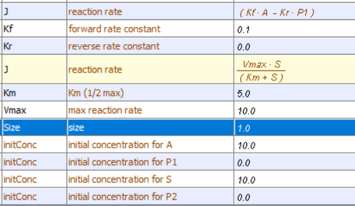
Initial Condition:  VM = 10  ; KM = 10;  S = 50	Initial Conditions: k1 = 10  ; k2 = 90 ;  k3 = 10 ;  E0 = 1 uM; S = 50 VM = k3E0 =10;   KM = (k2 + k3)/k2 = 10)

Select Load [model name] below

 Select Start to begin the simulation.

Interactive Element

Select Plot to change Y axis min/max, then Reset and Play  |  Select Slider to change which constants are displayed |  Select About  for software information.

Move the sliders to change the constants and see changes in the displayed graph in real-time.

Time course model made using Virtual Cell (Vcell), The Center for Cell Analysis & Modeling, at UConn Health.  Funded by NIH/NIGMS (R24 GM137787); Web simulation software (miniSidewinder) from Bartholomew Jardine and Herbert M. Sauro, University of Washington.  Funded by NIH/NIGMS (RO1-GM123032-04)

---

 

The initial conditions in the graph are set so the graphs of the rapid equilibrium and steady state are identical.

Recommendations:

• Scale the y-axis to 50
• change the slider k_{2_r2} for the steady state graph to other values. Watch the curves separate. Although these plots are for only one substrate concentration (50 uM), the effects of varying k₂ in the steady state plot are very dramatic. This should convince you that, in general, unless k₃ << k₂, the calculated value of K_M is not equal to the thermodynamic dissociation constant, K_D.

Analysis of the General Michaelis-Menten Equation

This equation can be simplified and studied under different conditions. First, notice that (k₂ + k₃)/k₁ is a constant, which is a function of relevant rate constants. This term is usually replaced by K_M, the Michaelis constant. Likewise, when S approaches infinity (i.e., S >> K_M, equation 5 becomes v = k₃(E₀), which is also a constant called V_M, the maximal velocity. Substituting V_M and K_M into equation 5 gives the simplified equation:

\begin{equation}
\mathrm{v}=\frac{\mathrm{V}_{\mathrm{M}}[\mathrm{S}]}{\mathrm{K}_{\mathrm{M}}+\mathrm{S}}
\end{equation}

It is extremely important to note that K_M in the general equation does not equal K_S, the dissociation constant used in the rapid equilibrium assumption! K_M and K_S have the same units of molarity, however. A closer examination of K_M shows that under the limiting case when k₂ >> k₃ (the rapid equilibrium assumption), then,

\begin{equation}
\mathrm{K}_{\mathrm{M}}=\frac{\mathrm{k}_2+\mathrm{k}_3}{\mathrm{k}_1}=\frac{\mathrm{k}_2}{\mathrm{k}_1}=\mathrm{K}_{\mathrm{D}}=\mathrm{K}_{\mathrm{S}}
\end{equation}

If we examine these equations under several different scenarios, we can better understand the equation and the kinetic parameters:

• when S = 0, v = 0.
• when S >> K_M, v = V_M = k₃E₀. (i.e., v is zero order with respect to S and first order in E. Remember, k₃ has units of s^-1> since it is a first-order rate constant. k₃ is often called the turnover number, because it describes how many molecules of S "turn over" to product per second.
• v = V_M2, when S = K_M.
• when S << K_M, v = V_MS/K_M = k₃E₀S/K_M (i.e., the reaction is bimolecular, dependent on both S and E. k₃/K_M has units of M^-1s^-1, the same as a second-order rate constant.

More Complicated Enzyme-catalyzed Reactions

A reversibly-catalyzed reaction

You previously learned that enzymes don't change the equilibrium constant for a reaction but rather decrease the activation energy barrier for both the forward and reverse reactions. This implies that the activation energy to move in the reverse direction, from products to reactants, is also lowered. Hence, the enzyme speeds up both the forward and reverse reactions. We haven't accounted for that in our kinetic equations yet. Many metabolic reactions with small negative ΔG values (i.e., not significantly favored) are reversible, allowing the enzyme to be used in the reverse direction. Take, for example, the pathway that breaks down glucose into pyruvate (glycolysis). It has nine steps, of which five are reversible, allowing them to be used in the reverse pathway to take pyruvate to glucose (gluconeogenesis).

Let's set up the equations for the reversible reaction of substrate S to product P catalyzed by enzyme E. Assume that the K_M for the forward reaction is K_MS (or K_S) and for the reverse reaction is K_MP (or K_P) as shown in the reaction scheme in Figure \(\PageIndex{2}\). The rate constant k₂ is the k_cat (forward rate constant) for conversion of ES to EP, and k_-2 is the k_cat (reverse rate constant) for conversion of EP to ES

Figure \(\PageIndex{2}\): Reaction scheme for a simple enzyme-catalyzed reaction

The following simple Michaelis-Menten equations can be written for just the forward reaction and for the reverse reaction:

\begin{equation}
\begin{aligned}
&v_f=\frac{V_f S}{K_{M S}+S}=\frac{\frac{V_f S}{K_{M S}}}{1+\frac{S}{K_{M S}}} \\
&v_r=\frac{V_r P}{K_{M P}+P}=\frac{\frac{V_r P}{K_{M P}}}{1+\frac{P}{K_{M P}}}
\end{aligned}
\end{equation}

You might think that simply subtracting the two would give the net velocity in the forward direction, but that is NOT the case.

\begin{equation}
v \neq\left[\frac{\frac{V_f S}{K_{M S}}}{1+\frac{S}{K_{M S}}}-\frac{\frac{V_r P}{K_{M P}}}{1+\frac{P}{K_{M P}}}\right]
\end{equation}

The reason is that, in the derivation, the equations for both the forward and reverse rates must include terms for the forward and reverse reactions, respectively.

A simple derivation shows that this is the equation for the reversible conversion of substrate to product.

\begin{equation}
v=k_2[E S]-k_{-2}[E P]=\frac{V_f \frac{[S]}{K_S}}{\left[1+\frac{[S]}{K_S}+\frac{[P]}{K_p}\right]}-\frac{V_r \frac{[P]}{K_P}}{\left[1+\frac{[S]}{K_S}+\frac{[P]}{K_P}\right]}=\frac{V_f \frac{[S]}{K_S}-V_r \frac{[P]}{K_P}}{\left[1+\frac{[S]}{K_S}+\frac{[P]}{K_P}\right]}
\end{equation}

This reversible form of the Michaelis-Menten equation and other equations, written in the format shown in equation 6.24, are commonly used in programs such as VCell and Copasi to model the kinetics of whole pathways of biological interactions and reactions. The figures below show a reaction diagram, graphical results of S and P vs. time for the selected K_M and V_M values, and animations of the reaction. The chemicals (S and P) are shown as green spheres connected by a line. The red dot again represents the enzyme (shown as a node with a connection between S and P). Equation 6.24 was used to model the reversible reaction (even though the arrows shown between S and P are unidirectional.

---

MODEL

Reversible Enzyme-Catalyzed Reaction:   E + S  ↔  ES  ↔  EP  ↔ E  + P .

Vcell reaction diagram (1-way arrows defined as reversible in the actual mathematical model) and chemical equation

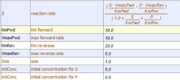
Initial parameter values: as shown in above

Select Load [Enz Rev] below

 Select Start to begin the simulation.

Interactive Element

Select Plot to change Y axis min/max, then Reset and Play  |  Select Slider to change which constants are displayed |  Select About  for software information.

Move the sliders to change the constants and see changes in the displayed graph in real-time.

Time course model made using Virtual Cell (Vcell), The Center for Cell Analysis & Modeling, at UConn Health.  Funded by NIH/NIGMS (R24 GM137787); Web simulation software (miniSidewinder) from Bartholomew Jardine and Herbert M. Sauro, University of Washington.  Funded by NIH/NIGMS (RO1-GM123032-04)

---

 

If you reflect on it, this reaction is very similar to the reversible reaction of A ↔ P in the absence of an enzyme, which we explored in Chapter section 6.2. Just for comparison, the graph for that reaction is shown below. Change the sliders to produce a curve similar to the enzyme-catalyzed reaction shown in the figure above.

Reaction with intermediates

Not all reactions can be characterized simply as a substrate interacting with an enzyme to form an ES complex, which then turns over to form the product. Sometimes, intermediates form. For example, a substrate S might interact with E to form a complex, which is then cleaved into products P and Q. Q is released from the enzyme, whereas P may remain covalently bound. This often occurs during the hydrolytic cleavage of a peptide bond by a protease, when an activated nucleophile, such as serine, reacts with the sessile peptide bond in a nucleophilic substitution reaction, releasing the amine end of the former peptide as the leaving group. The carboxy end of the peptide bond remains bonded to the Ser as a Ser-acyl intermediate. Water then enters and cleaves the acyl intermediate, freeing the carboxyl end of the original peptide bond. This is shown in the written reaction in Figure \(\PageIndex{3}\):

Figure \(\PageIndex{3}\): Reaction scheme for enzyme-catalyzed reaction with an intermediate

Even for this seemingly complicated reaction, you get the standard Michaelis-Menten equation.

To simplify the derivation of the kinetic equation, let's assume that E, S, and ES are in rapid equilibrium defined by the dissociation constant, Ks. Assume Q has a visible absorbance, so it is easy to monitor. Assume from the steady state assumption that:

\begin{equation}
\frac{\mathrm{d}[\mathrm{E}-\mathrm{P}]}{\mathrm{dt}}=\mathrm{k}_2[\mathrm{ES}]-\mathrm{k}_3[\mathrm{E}-\mathrm{P}]=0
\end{equation}

assuming that k₃ is a pseudo first-order rate constant and that [H₂O] doesn't change.

The velocity depends on which step is rate-limiting. If k₃ << k₂, then the k₃ step is rate-limiting. Then

\begin{equation}
\mathrm{v}=\mathrm{k}_3[\mathrm{E}-\mathrm{P}]
\end{equation}

If k₂ << k₃, then the k₂ step is rate-limiting. Then

\begin{equation}
\mathrm{v}=\mathrm{k}_2[\mathrm{ES}]
\end{equation}

The following kinetic equation for this reaction can be derived, assuming v = k₂[ES].

\begin{equation}
\mathrm{v}=\frac{\frac{\mathrm{k}_2 \mathrm{k}_3}{\mathrm{k}_2+\mathrm{k}_3}\left[\mathrm{E}_0\right][\mathrm{S}]}{\left(\frac{\mathrm{k}_3}{\mathrm{k}_2+\mathrm{k}_3}\right) \mathrm{K}_{\mathrm{S}}+\mathrm{S}}=\frac{\mathrm{k}_{\mathrm{cat}}\left[\mathrm{E}_0\right][\mathrm{S}]}{\mathrm{K}_{\mathrm{M}}+\mathrm{S}}=\frac{\mathrm{V}_{\mathrm{M}} \mathrm{S}}{\mathrm{K}_{\mathrm{M}}+\mathrm{S}}
\end{equation}

You can verify that you get the same equation if you assume that v = k₃[E-P].

This equation looks quite complicated, especially if you substitute for Ks, k_-1/k₁. All the kinetic constants can be expressed as functions of the individual rate constants. However, this equation can be simplified by realizing the following:

• When \(\mathrm{S}>>\frac{\mathrm{K}_{\mathrm{S}} \mathrm{k}_{3}}{\mathrm{k}_{2}+\mathrm{k}_{3}}, \mathrm{v}=\left(\frac{\mathrm{k}_{2} \mathrm{k}_{3}}{\mathrm{k}_{2}+\mathrm{k}_{3}}\right) \mathrm{E}_{0}=\mathrm{V}_{\mathrm{M}}\)
• \(\frac{\mathrm{K}_{\mathrm{S}} \mathrm{k}_{3}}{\mathrm{k}_{2}+\mathrm{k}_{3}}=\mathrm{constant}=\mathrm{K}_{\mathrm{M}}\)

Substituting these into equation 7 gives:

\[\mathrm{v}=\frac{\mathrm{V}_{\mathrm{M}} \mathrm{S}}{\mathrm{K}_{\mathrm{M}}+\mathrm{S}} \nonumber \]

This, again, is the general form of the Michaelis-Menten equation

The expression for V_M in the first bulleted expression above is more complicated than our earlier definition of V_M = k₃E₀. They are similar in that the term E₀ is multiplied by a constant, which is itself a function of rate constant(s). The rate constants are generally lumped into a single generic constant, k_cat.

• For the simple reaction k_cat = k3
• For the more complicated reaction above with a covalent intermediate, \(\mathrm{k}_{\mathrm{cat}}=\frac{\mathrm{k}_{2} \mathrm{k}_{3}}{\mathrm{k}_{2}+\mathrm{k}_{3}}\)
• For all reactions, V_M = k_catE₀.

Recent Updates (2/7/24): Here is a VCell computational model for a bisubstrate, biproduct (BiBi) reaction with a covalent intermediate (ping-pong reaction).

---

MODEL

BiBi-Ping Pong_Covalent Intermediate Irreversible reaction

Vcell reaction diagram (1-way arrows defined as reversible in actual mathematical model) and chemical equation

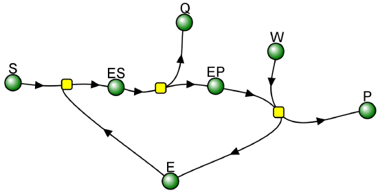
Yellow dots: Reaction Nodes (R1, R2 and R3 left to right)

Reaction made irreversible since k_r2 = 0, k_r3 = 0.

Initial parameter values:

• S₀ = 100, E₀ = 1, W (water in a hydrolysis reaction) = 50 and fixed throughout
• k_1f = 5, k_1r = 1, k_2f = 0.6,
• k_2f = 50, k_2r = 0
• k_3f = 0.05, k_3f = 0

Select Load [model name] below

 Select Start to begin the simulation.

1Interactive Element

Select Plot to change Y axis min/max, then Reset and Play  |  Select Slider to change which constants are displayed |  Select About  for software information.

To see the burst phase for reaction, change the time and parameters to these values:

• set Run time to 0.3
• Select Plot then Update Y axis max to 2
• Click Edit Plot Species and check just P and Q
• reset

Time course model made using Virtual Cell (Vcell), The Center for Cell Analysis & Modeling, at UConn Health.  Funded by NIH/NIGMS (R24 GM137787); Web simulation software (miniSidewinder) from Bartholomew Jardine and Herbert M. Sauro, University of Washington.  Funded by NIH/NIGMS (RO1-GM123032-04)

---

 

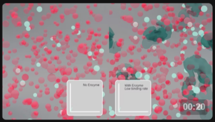
When k₂ >> k₃, Q forms quickly in a burst phase due to a high k₂.  This phase is followed by the slower conversion of the accumulated EP to E + P in a steady state phase, as shown below in Figure \(\PageIndex{4}\).  Make sure to change the parameters in the model above to see the burst phase for the production of product Q.  This reaction is an example of a BiBi (two substrates, two products) Ping Pong reaction, since one reactant binds, followed by one product departing before the second reactant binds and the second product departs.

Figure \(\PageIndex{4}\): Burst and steady-state phase in an enzyme-catalyzed reaction with a covalent intermediate and k₂ >> k₃. 

Reverse the rate constants in the model to k₂ = 5 and  k₃ = 0.5 so that  k₂ is not >> k_3, and note that the burst phase for Q disappears!

When plotting v₀ vs S Michaelis-Menten plots of this type of reaction, the steady state v₀ should be used and NOT (v₀) _t=0 = (dQ/dt) _t=0, since that rate changes very quickly with the initial burst formation of Q.

Summary to this point

Figure \(\PageIndex{5}\) compares the Michaelis-Menten kinetic equations for the rapid equilibrium, steady state assumptions, and covalent intermediate cases.

Figure \(\PageIndex{5}\): Michaelis-Menten kinetic equations for the rapid equilibrium, steady state assumptions, and covalent intermediate cases

Meaning of Kinetic Constants

Getting a "gut-level" understanding of the significance of the rate constants is important. Here they are:

• K_M: The Michaelis constant, with units of molarity (M), is operationally defined as the substrate concentration at which the initial velocity is half of V_M. It is equal to the dissociation constant of E and S only if E, S, and ES are in rapid equilibrium. It can be thought of as an "effective" (but not actual) K_D in other cases.
• k_cat: The catalytic rate constant, with units of s^-1, is often called the turnover number. It is a measure of how many bound substrate molecules "turnover" or form product in 1 second. This is evident from equation v₀ = k_cat[ES]
• k_cat/K_M: Under condition when [S] << K_M, the Michaelis-Menten equation becomes v₀ = (k_cat/K_M)[E₀][S]. This really describes a biomolecular rate constant (k_cat/K_M), with units of M^-1s^-1, for the conversion of free substrate to product. Some enzymes have k_cat/K_M values around 10⁸, indicating they are diffusion-controlled. That implies the reaction occurs essentially as soon as the enzyme and substrate collide. The constant k_cat/K_M is also called the specificity constant, as it describes how well an enzyme distinguishes between competing substrates. (We will show this mathematically in the next chapter.)

Table \(\PageIndex{1}\) below shows K_M and k_cat values for various enzymes

KM values
enzyme	substrate	Km (mM)
catalase	H2O2	25
hexokinase (brain)	ATP	0.4
	D-Glucose	0.05
	D-Fructose	1.5
carbonic anhydrase	HCO3^-	9
chymotrypsin	glycyltyrosinylglycine	108
	N-benzoyltyrosinamide	2.5
b-galactosidase	D-lactose	4.0
threonine dehydratase	L-Thr	5.0
kcat values
enzyme	substrate	kcat (s^-1)
catalase	H2O2	40,000,000
carbonic anhydrase	HCO3^-	400,000
acetylcholinesterase	acetylcholine	140,000
b-lactamase	benzylpenicillin	2,000
fumarase	fumarate	800
RecA protein (ATPase)	ATP	0.4

Table \(\PageIndex{1}\): K_M and k_cat values for various enzymes

Table \(\PageIndex{2}\) below shows k_cat, K_M, and k_cat/K_M values for diffusion-controlled enzymes

Enzymes with kcat/KM values close to diffusion-controlled (10^8 - 10^9 M^-1s^-1)
enzyme	substrate		kcat (s^-1)	Km (M)	kcat/Km (M^-1s^-1)
acetylcholinesterase	acetylcholine		1.4 x 10^4	9 x 10^-5	1.6 x 10^8
carbonic anhydrase	CO2		1 x 10^6	1.2 x 10^-2	8.3 x 10^7
	HCO3^-		4 x 10^5	2.6 x 10-2	1.5 x 10^7
catalase	H2O2		4 x 10^7	1.1	4 x 10^7
crotonase	crotonyl-CoA		5.7 x 10^3	2 x 10^-5	2.8 x 10^8
fumarase	fumarate		8 x 10^2	5 x 10^-6	1.6 x 10^8
	malate		9 x 10^2	2.5 x 10^-5	3.6 x 10^7
triose phosphate isomerase	glyceraldehyde-3-P		4.3 x 10^3	4.7 x 10^-4	2.4 x 10^8
b-lactamase	benzylpenicillin		2.0 x 10^3	2 x 10^-4	1 x 10^8

Table \(\PageIndex{2}\) below shows k_cat, K_M and k_cat/K_M values for diffusion-controlled enzymes

Experimental Determination of V_M and K_M

How can V_M and K_M be determined from experimental data?

From the initial rate data

The most common way to determine V_M and K_M is by using the initial rates, v₀, obtained from P or S vs. time curves. Hyperbolic graphs of v₀ vs [S] can be fitted or transformed, as we explored the different mathematical transformations of the hyperbolic binding equation to determine K_D. These included:

• Michaelis-Menten plot: nonlinear hyperbolic fit
• Lineweaver-Burk double reciprocal plot
• Scatchard plot
• Eadie-Hofstee plot

We discussed all of these plots, except for the Eadie-Hofstee plot, in the chapter on binding. The Eadie-Hofstee plot is another linearized version of the Michaelis-Menten equation

Here is a derivation of that equation, which starts with each side of the double-reciprocal plot being multiplied by v₀V_M.

\begin{equation}
\begin{aligned}
\left(v_0 V_M\right) \frac{1}{v_0} &=\left(v_0 V_M\right)\left(\frac{K_M}{V_M}\right) \frac{1}{S}+\left(v_0 V_M\right) \frac{1}{V_M} \\
V_M &=\left(v_0\right) K_M \frac{1}{S}+\left(v_0\right) \\
v_0 &=-K_M\left(\frac{v_0}{S}\right)+V_M
\end{aligned}
\end{equation}

Note that a graph of v₀ vs v₀/S is linear, so the slope and intercept can be used to obtain values for V_M and K_M.

The double-reciprocal plot is commonly used to analyze initial velocity vs substrate concentration data. When used for such purposes, the graphs are referred to as Lineweaver-Burk plots, where plots of 1/v vs 1/S are straight lines with slope m = K_M/V_M, and y-intercept b = 1/V_M. Figure \(\PageIndex{6}\) common graphs used to display initial rate enzyme kinetic data.

Figure \(\PageIndex{6}\): Common graphs used to display initial rate enzyme kinetic data

The straight-line plots shown above should not be analyzed using linear regression, as linear regression assumes constant error in the v₀ values. A weighted linear regression or, even better, a nonlinear fit to a hyperbolic equation should be used. (Common Error in Biochemistry Textbooks: The Shape of the Hyperbola). A rearrangement of the corresponding Scatchard equations to their equivalent form in kinetics, the Eadie-Hofstee plot. is also commonly used, especially to visualize enzyme inhibition data, as we will see in the next chapter.

An Extension: k_cat and V_M from integrated rate equations

K_M and V_M could be theoretically extracted from progress curves of A or P as a function of t at one single A concentration by deriving an integrated rate equation for A or P as a function of t, as we did in equation 2 (the integrated rate equation for the conversion of A → P in the absence of enzyme). In principle, this method would be better than the initial rate method. Why? It is not easy to be certain that you are measuring the initial rate for each [S], which should vary widely. It's also time-intensive. In addition, consider how much data is discarded when you measure the entire progress curve at each substrate concentration, especially if you quench the reaction at a single time point, effectively limiting the data to a single time point per substrate.

In practice, the mathematics is complicated, and it is impossible to obtain a simple, explicit expression for [P] or [S] as functions of time. A slight variant of a progress curve can be derived. Let us consider the simple case of a single substrate S (or A) being converted to product P in an enzyme-catalyzed reaction. The analogous equations for first-order, noncatalyzed rates were A=A₀e^-k₁t or P = A₀(1-e^-k₁t).

We can derive the equation for the enzyme-catalyzed reaction shown below.

Here it is!

\begin{equation}
\frac{\mathrm{P}}{\mathrm{t}}=\frac{\mathrm{K}_{\mathrm{M}} \ln \left(\frac{\mathrm{S}_0-\mathrm{P}}{\mathrm{S}_0}\right)}{\mathrm{t}}+\mathrm{V}_{\mathrm{M}}
\end{equation}

Derivation: k_cat and V_M from integrated rate equation

Click below to see the derivation

Derivation

\begin{equation}
\begin{array}{r}
\mathrm{v}=-\frac{\mathrm{dS}}{\mathrm{dt}}=+\frac{\mathrm{dP}}{\mathrm{dt}}=\frac{\mathrm{V}_{\mathrm{M}} \mathrm{S}}{\mathrm{K}_{\mathrm{M}}+\mathrm{S}} \\
\int_{\mathrm{S}_0}^{\mathrm{S}} \frac{\mathrm{K}_{\mathrm{M}}+\mathrm{S}}{\mathrm{V}_{\mathrm{M}} \mathrm{S}} \mathrm{d} S=-\int_0^{\mathrm{t}} \mathrm{t}
\end{array}
\end{equation}

\begin{equation}
-\mathrm{t}=\frac{\mathrm{S}+\mathrm{K}_{\mathrm{M}} \ln \mathrm{S}-\mathrm{S}_0-\mathrm{K}_{\mathrm{M}} \ln S_0}{\mathrm{~V}_{\mathrm{M}}}
\end{equation}

On rearrangement, this gives:

\begin{equation}
\mathrm{S}_0-\mathrm{S}+\mathrm{K}_{\mathrm{M}} \ln \frac{\mathrm{S}_0}{\mathrm{~S}}=\mathrm{V}_{\mathrm{M}} \mathrm{t}
\end{equation}

This equation is an implicit equation, not an explicit one, as it does NOT give S(t) explicitly as a function of t.

Equation yy can be written with respect to product P as follows:

\begin{equation}
\begin{aligned}
&P=\mathrm{S}_0-S{ }^{\prime \prime} \text { or }{ }^{\prime \prime} S=\mathrm{S}_0-P \\
&\mathrm{~S}_0-\left(\mathrm{S}_0-\mathrm{P}\right)+\mathrm{K}_{\mathrm{M}} \ln \frac{\mathrm{S}_0}{\mathrm{~S}_0-\mathrm{P}}=\mathrm{V}_{\mathrm{M}} \mathrm{t} \\
&\mathrm{P}-\mathrm{K}_{\mathrm{M}} \ln \left(\frac{\mathrm{S}_0-\mathrm{P}}{\mathrm{S}_0}\right)=\mathrm{V}_{\mathrm{M}} \mathrm{t}
\end{aligned}
\end{equation}

Rearranging this gives

\begin{equation}
\frac{\mathrm{P}}{\mathrm{t}}=\frac{\mathrm{K}_{\mathrm{M}} \ln \left(\frac{\mathrm{S}_0-\mathrm{P}}{\mathrm{S}_0}\right)}{\mathrm{t}}+\mathrm{V}_{\mathrm{M}}
\end{equation}

S(t) explicitly as a function of t.

This equation does not give P(t) explicitly as a function of time. Rather, one can obtain a graph of P/t vs [ln (1-P/S₀)]/t (shown below) from the derived equation, which yields a straight line with a slope of K_M and a y-intercept of V_M. Note that the calculated values of V_M and K_M are derived from only one substrate concentration, and the values may be affected by product inhibition.

Figure \(\PageIndex{7}\) compares a first-order noncatalyzed conversion of A → P to the enzyme-catalyzed rate. The V_M for the enzyme-catalyzed reaction was chosen to be small to make the two graphs comparable.

Figure \(\PageIndex{7}\): Comparison of a first order noncatalyzed conversion of A → P to the enzyme catalyzed rate

Note that the curves are similar but not identical. If you didn't know an enzyme was present, you could fit the data to a first-order rise in [P] with time, but it would not be the optimal fit. The progress curves are much more complicated to analyze if the product, which shares structural similarities with the substrate, binds the enzyme tightly and inhibits it (product inhibition).

Comparison of Progress Curves for Uncatalyzed and Catalyzed Reactions.

Let's explore progress curves for enzyme-catalyzed reactions a bit further. Students usually see v₀ vs. [S] Michaelis-Menten plots in textbooks. These plots are, in some ways, less intuitive than seeing P vs. t curves, which are more in line with how we might contemplate how a reaction proceeds. Hence, it would be illuminating to compare progress curve graphs of A → P (irreversible) for the uncatalyzed and S → P for the enzyme-catalyzed reactions. What might you expect? We saw one example in Figure \(\PageIndex{6}\).

In each case, P should increase with time. In the uncatalyzed reaction, S exponentially decreases to 0, and P rises to P = S₀. You also see a rise in P vs t for the enzyme-catalyzed rate, but you would expect a faster rise over time since the enzyme catalyzes the reaction. Figure \(\PageIndex{87}\) shows a comparison of the progress curves for the uncatalyzed first-order reaction of A → P₁ (red) and S → P₂ (blue) for the enzyme-catalyzed reaction (blue, right) for these conditions: uncatalyzed reaction A → P₁, k₁ = 0.1; Catalyzed reaction: S → P₂, V_M=10, K_M=5. Note that the rate at which bound S (i.e, ES) goes to P for the catalyzed rate is 100x faster than the rate constant for the catalyzed rate.

Figure \(\PageIndex{8}\): Another comparison of progress curves (P vs t) for a catalyzed and uncatalyzed conversion of A → P.

Note that the curves are somewhat similar in shape but also clearly different in comparison to the one shown in Figure \(\PageIndex{6}\).

Now, let's use Vcell to compare the reactions for different values of the kinetic constants for the uncatalyzed and the enzyme-catalyzed reactions. Change the constants and find a set of conditions so that the catalyzed and uncatalyzed rates for the conversion of reactants to products are superimposable. How can that be?

---

MODEL

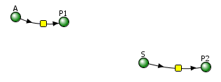
Irreversible reactions:  A → P1  and E + S ↔ ES → E + P 

Vcell reaction diagram (1-way arrows defined as reversible in actual mathematical model) and chemical equation

Initial conditions

Select Load [model name] below

 Select Start to begin the simulation.

Interactive Element

Select Plot to change Y axis min/max, then Reset and Play  |  Select Slider to change which constants are displayed |  Select About  for software information.

Move the sliders to change the constants and see changes in the displayed graph in real-time.

Time course model made using Virtual Cell (Vcell), The Center for Cell Analysis & Modeling, at UConn Health.  Funded by NIH/NIGMS (R24 GM137787); Web simulation software (miniSidewinder) from Bartholomew Jardine and Herbert M. Sauro, University of Washington.  Funded by NIH/NIGMS (RO1-GM123032-04)

---

 

Animations

Now let's look at an animation of the same irreversible reactions in which the enzyme-catalyzed reaction is no faster than the noncatalyzed rate (a worthless enzyme!). Here are the reactions:

A→P, k₁ =0.1; S → P, V_M=?, K_M = ?.

The animations show just the accumulation of products. Animations are by Shraddha Nakak and Hui Liu.

Exercise \(\PageIndex{1}\)

Use the Vcell model above to find a set of values for K_M and V_M that would make the two graphs superimposable - i.e., when the graphs in the absence and presence of E are identical. (Hint: that would be a really bad enzyme if it didn't increase the reaction over the uncatalyzed rate!)

Answer

K_M = 96, V_M = 10

Summary

(Summary written by Claude, Sonnet 4.6, Anthropic)

This chapter develops the mathematical framework for enzyme kinetics — the quantitative description of how enzyme-catalyzed reaction rates depend on substrate concentration — progressing from the simpler rapid-equilibrium derivation through the more general steady-state treatment, to extensions to reversible reactions and covalent intermediates, and to the practical methods used to extract kinetic parameters from experimental data.

The enzyme kinetics problem begins with the observation that enzymes lower the activation energy without changing the equilibrium constants, thereby accelerating both the forward and reverse reactions. The simplest kinetic scheme is E + S ⇌ ES → E + P, in which the enzyme E binds substrate S to form the complex ES, which then undergoes chemical transformation to release product P and regenerate free enzyme. Two complementary mathematical approaches — initial rate analysis (measuring v₀ as a function of [S]₀) and progress curve analysis (monitoring [P] or [S] as a function of time) — are used to characterize this reaction.

The rapid equilibrium derivation assumes that k₂ >> k₃, so that ES reaches thermodynamic equilibrium with E and S before significant product forms. Under this assumption, [ES] is determined by the dissociation constant K_S = k₂/k₁, and the initial velocity is v₀ = k₃[ES]. Using mass balance (E₀ = [E] + [ES]) and the expression for [ES] in terms of K_S, [E₀], and [S], one obtains the Henri-Michaelis-Menten equation: v₀ = V_M[S]/(K_S + [S]), more typically written as v₀ = V_M[S]/(K_M + [S]), where V_M = k₃E₀ and K_M is the Michaelis constant. This equation is a rectangular hyperbola with the same mathematical form as the ligand-binding equation, with K_S playing the role of K_D. Under rapid equilibrium conditions, K_M = K_S is the true thermodynamic dissociation constant for the ES complex.

The steady state derivation relaxes the requirement that k₂ >> k₃, instead assuming only that d[ES]/dt ≈ 0 — that ES accumulates to a quasi-constant level within milliseconds that persists throughout the initial rate measurement. Setting d[ES]/dt = k₁[E][S] − k₂[ES] − k₃[ES] = 0 and solving using mass balance gives the same hyperbolic equation but with K_M = (k₂ + k₃)/k₁. This K_M is not equal to the thermodynamic dissociation constant K_S = k₂/k₁ unless k₂ >> k₃ (the rapid equilibrium limit). The general K_M is therefore an operational parameter — the substrate concentration at which v₀ = V_M/2 — that should not be interpreted as a thermodynamic binding constant in the general case. VCell simulations confirm that changing k₂ relative to k₃ separates the rapid-equilibrium and steady-state progress curves, demonstrating that K_M ≠ K_S unless the rapid-equilibrium condition holds.

Interpreting the kinetic parameters requires understanding their physical meaning. K_M (units: M) is operationally defined as the substrate concentration at half-maximal velocity; it reflects both binding affinity and the relative rates of ES breakdown pathways. The turnover number kcat (units: s⁻¹) measures how many substrate molecules one active site converts to product per second at saturating substrate, ranging from ~0.4 s⁻¹ for RecA ATPase to 4 × 10⁷ s⁻¹ for catalase. V_M = kcat × E₀ is the maximal velocity, proportional to total enzyme concentration. The specificity constant kcat/K_M (units: M⁻¹s⁻¹) is the apparent second-order rate constant for the reaction of free E with free S when [S] << K_M; it determines how effectively an enzyme discriminates between competing substrates and reaches the diffusion-controlled limit of ~10⁸–10⁹ M⁻¹s⁻¹ for the most efficient enzymes (triose phosphate isomerase, carbonic anhydrase, acetylcholinesterase, catalase, fumarase).

Covalent intermediates add mechanistic richness. For a reaction in which substrate S is cleaved to release Q immediately but P remains covalently attached as an enzyme-acyl intermediate (E-P), then hydrolyzed by water to release P and regenerate E, the same hyperbolic Michaelis-Menten equation results, but with k_cat = k₂k₃/(k₂ + k₃) — the harmonic mean rate constant reflecting two sequential first-order steps. When k₂ >> k₃, a transient burst phase of rapid Q formation occurs as E-P accumulates before the slower hydrolytic k₃ step becomes rate-limiting. The steady-state phase, not the burst phase, should be used for Michaelis-Menten analysis of such reactions, since only the steady-state v₀ follows the standard v₀ vs. [S] hyperbola.

Reversible enzyme-catalyzed reactions — important for the many metabolic enzymes with modestly negative ΔG° that operate reversibly in vivo — require a unified rate equation in which both forward and reverse velocity terms are correctly coupled. The net forward rate is not simply v_forward − v_reverse, but is given by a single equation with terms for K_MS (K_M for substrate), K_MP (K_M for product), V_M(forward), and V_M(reverse). This reversible Michaelis-Menten equation is the form used in whole-pathway kinetic simulations in programs such as VCell and COPASI.

Experimental determination of V_M and K_M uses the initial velocity method, in which v₀ values at varying [S] are fit to the Michaelis-Menten hyperbola by nonlinear regression. Linearizing transformations — the Lineweaver-Burk double-reciprocal plot (1/v₀ vs. 1/[S], slope = K_M/V_M, y-intercept = 1/V_M), the Scatchard plot, and the Eadie-Hofstee plot (v₀ vs. v₀/[S], slope = −K_M, y-intercept = V_M) — are useful for visualizing data and detecting inhibition patterns but are statistically inferior to nonlinear fitting because linear transformation propagates error non-uniformly. Progress curve analysis, using the integrated Michaelis-Menten equation which yields a linear plot of [P]/t vs. ln(1 − [P]/S₀)/t with slope K_M and y-intercept V_M, can in principle extract both parameters from a single progress curve at one substrate concentration, but is complicated by product inhibition and the lack of an explicit [P] = f(t) solution