6.4: Enzyme Inhibition

Search Fundamentals of Biochemistry

Learning Goals (ChatGPT o1, 1/30/25)

(Learning goals written by Claude, Sonnet 4.6, Anthropic)

Reversible Inhibition: Mechanisms and Kinetic Signatures

• Distinguish competitive, uncompetitive, and noncompetitive/mixed inhibition mechanisms by describing where the inhibitor binds (free E only for competitive; ES only for uncompetitive; both E and ES for mixed/noncompetitive), and predict the effect of each mechanism on K_Mapp and V_Mapp — using Le Chatelier's principle to rationalize why competitive inhibition increases K_Mapp while leaving V_M unchanged, uncompetitive inhibition decreases both K_Mapp and V_Mapp by the same factor (1 + I/K_ii), and noncompetitive inhibition decreases V_Mapp while leaving K_M unchanged.
• Interpret Lineweaver-Burk double-reciprocal plots for each inhibition type — recognizing the hallmark patterns of lines intersecting on the y-axis (competitive, same 1/V_M), parallel lines with changed intercepts (uncompetitive), and lines intersecting on the x-axis (noncompetitive) — and use slopes and intercepts to extract K_IS and/or K_ii from experimental data.
• Write and apply the modified Michaelis-Menten velocity equations for each inhibition type: v₀ = V_M[S]/(K_M(1 + I/K_IS) + [S]) for competitive inhibition, where K_Mapp = K_M(1 + I/K_IS); v₀ = V_M[S]/(K_M + [S](1 + I/K_ii)) for uncompetitive inhibition, where both K_Mapp = K_M/(1 + I/K_ii) and V_Mapp = V_M/(1 + I/K_ii); and the mixed equation where both K_Mapp and V_Mapp change with inhibitor concentration governed by K_IS and K_ii independently.
• Explain the concept of the specificity constant k_cat/K_M in the context of competing substrates — deriving that the ratio of initial velocities for two competing substrates at equal concentration equals the ratio of their k_cat/K_M values — and use this relationship to explain how an enzyme selects among multiple substrates in vivo.

Special Cases and Physiological Contexts

• Explain product inhibition as a special case of competitive inhibition in which the structurally similar product P occupies the active site and inhibits further turnover of S, describe its effect on progress curves (downward curvature at early time points when product accumulates), and distinguish this from simple reversible product release.
• Contrast in vitro inhibition analysis (fixed enzyme, varying S at several fixed I concentrations, independent variable is [S]) with in vivo inhibition (enzyme embedded in a metabolic pathway with relatively constant flux v, where S concentration is determined by v rather than varied independently) — deriving that under constant flux conditions, competitive inhibition gives a linear relationship between S/K_M and I/K_IS whereas uncompetitive inhibition causes S/K_M to "blow up" to infinity at I = K_ii — and explain why this makes uncompetitive inhibitors theoretically more effective at disrupting metabolic pathways in vivo than competitive inhibitors.
• Explain how pH and temperature affect enzyme activity by altering the protonation states of catalytically essential active site residues (affecting k_cat), substrate binding (affecting K_M), and global protein conformation (affecting both), and identify which amino acid side chains are plausible candidates for the pH-sensitive residues in enzymes whose activity profiles peak at specific pH values.

 

Irreversible Covalent Inhibition

Given what you already know about protein structure, it should be easy to determine how to inhibit an enzyme. Since structure mediates function, anything that significantly alters an enzyme's structure would inhibit its activity. Hence, extremes of pH and high temperature, both of which can denature the enzyme, would irreversibly inhibit it unless it could refold properly. Alternatively, we could add a small molecule that interacts noncovalently with the enzyme, either altering its conformation or directly preventing substrate binding. Finally, we could covalently modify certain side chains, which, if they are essential to enzymatic activity, would irreversibly inhibit the enzyme.

We previously discussed the types of reagents that could chemically modify specific side chains critical to enzymatic activity. For example, iodoacetamide might abolish enzyme activity if a cysteine side chain is required. However, these reagents will usually modify several side chains. Determining which is critical for the binding or catalytic conversion of the substrate can be difficult. One way would be to protect the active site with saturating concentrations of a reversible-binding ligand. Then, the chemical modification can be performed at varying reaction times. The critical side chain would be protected from chemical modification, with the extent of protection determined by the K_D, the concentration of the protecting ligand, and the reaction time.

The rest of the chapter will deal with reversible, noncovalent inhibition

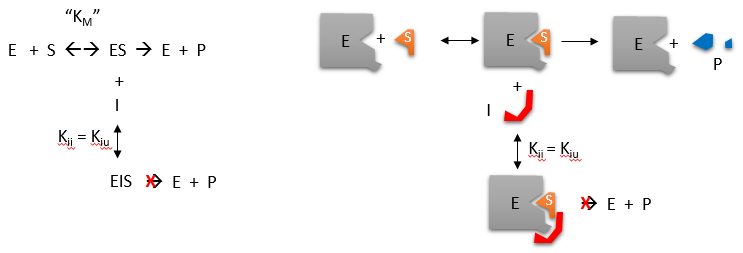
Competitive Inhibition

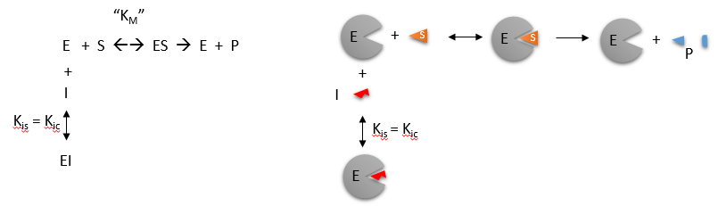
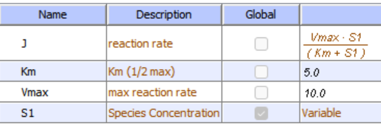
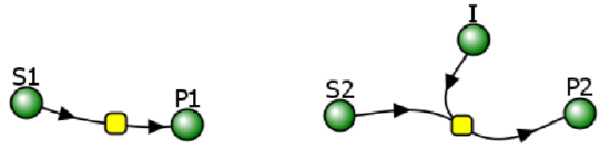
Reversible Competitive inhibition occurs when the substrate (S) and the inhibitor (I) bind to the same site on the enzyme. In effect, they compete for the active site and bind in a mutually exclusive fashion. This is illustrated in the chemical equations and molecular cartoons shown in Figure \(\PageIndex{1}\).

Figure \(\PageIndex{1}\): Competitive Inhibition

\begin{equation}
v_0=\frac{V_M S}{K_M\left(1+\frac{I}{K is}\right)+S}
\end{equation}

There is another type of inhibition that would give the same kinetic data. If S and I were bound to different sites, and S was bound to E and produced a conformational change in E such that I could not bind (and vice versa), then the binding of S and I would be mutually exclusive. This is called allosteric competitive inhibition. Inhibition studies are usually performed at several fixed, non-saturating I concentrations and varying S concentrations.

The key kinetic parameters to understand are V_M and K_M. Let us assume for ease of equation derivation that I binds reversibly and with rapid equilibrium to E, with a dissociation constant K_IS. The "s" in the subscript "is" indicates that the slope of the 1/v vs. 1/S Lineweaver-Burk plot changes while the y-intercept stays constant. K_IS is also named K_IC, where the subscript "c" stands for competitive inhibition constant.

A look at the top mechanism shows that even in the presence of I, as S increases to infinity, all E is converted to ES. That is, there is no free E to which I could bind. Now, remember that V_{M ,}= k_catE₀. Under these conditions, ES = E₀; hence, v = V_M. V_M is not changed. However, the apparent K_M, K_Mapp, will change. We can use LaChatelier's principle to understand this. If I binds to E alone and not ES, it will shift the equilibrium of E + S → ES to the left. This would increase the K_Mapp (i.e., it would appear that the affinity of E and S has decreased). The double reciprocal plot (Lineweaver-Burk plot) offers a great way to visualize the inhibition as shown in Figure \(\PageIndex{2}\).

Figure \(\PageIndex{2}\): Competitive Inhibition: Lineweaver-Burk plots

In the presence of I, V_M does not change, but K_M appears to increase. Therefore, 1/K_M, the x-intercept on the plot, will get smaller and closer to 0. Therefore, the plots will consist of a series of lines, with the same y-intercept (1/V_M), and the x-intercepts (-1/K_M) move closer to 0 as I increases. These intersecting plots are the hallmarks of competitive inhibition.

Here is an interactive graph showing v₀ vs [S] for competitive inhibition with Vm and Km both set to 100. Change the sliders for [I] and K_is and see the effect on the graph.

Here is the interactive graph showing 1/v₀ vs 1/[S] for competitive inhibition, with Vm and Km both set to 10.

Note that in the first three inhibition models discussed in this section, the Lineweaver-Burk plots are linear in the presence and absence of an inhibitor. This suggests that plots of v vs. S in each case would be hyperbolic and conform to the Michaelis-Menten equation, with potentially different apparent V_M and K_M values.

An equation for v₀ in the presence of a competitive inhibitor is shown in the above figure. The only change from the equation for the initial velocity in the absence of the inhibitor is that the K_M term is multiplied by 1 + I/K_is. Hence K_Mapp = K_M(1+I/Kis). This shows that the apparent K_M does increase as we predicted. K_IS is the inhibitor dissociation constant. The apparent K_M changes with increasing I, which affects the slope of the double reciprocal plot.

v₀ vs log [Inhibitor] plots

If the data were plotted as v₀ vs. log S, the plots would be sigmoidal, as we saw for plots of ML vs. log L in Chapter 5B. In the case of a competitive inhibitor, the plot of v₀ vs log S in the presence of different fixed concentrations of inhibitor would consist of a series of sigmoidal curves, each with the same V_M, but with different apparent K_M values (where K_Mapp = K_M(1+I/K_is), progressively shifted to the right. Enzyme kinetic data is rarely plotted this way. These plots are mostly used for simple binding data for the M + L ↔ ML equilibrium in the presence of different inhibitor concentrations.

Reconsider our discussion of the simple binding equilibrium, M + L ↔ ML. For fractional saturation Y vs a log L graphs, we considered three examples:

1. L = 0.01 K_D (i.e., L << K_D), which implies that K_D = 100L. Then Y = L/[K_D+L] = L/[100L + L] ≈1/100. This implies that irrespective of the actual [L], if L = 0.01 K_D, then Y ≈0.01.
2. L = 100 K_D (i.e,. L >> K_D), which implies that K_D = L/100. Then Y = L/[K_D+L] = L/[(L/100) + L] = 100L/101L ≈ 1. This implies that irrespective of the actual [L], if L = 100 Kd, then Y ≈1.
3. L = K_D, then Y = 0.5

These scenarios show that if L varies over four orders of magnitude (0.01K_D < K_D < 100K_D), or, in log terms, from
-2 + log K_D < log K_D< 2 + log K_D), irrespective of the magnitude of the K_D, that Y varies from approximately 0 - 1.

In other words, Y varies from 0 to 1 when L varies from log K_D by +2. Hence, plots of Y vs log L for a series of binding reactions of increasingly higher K_D (lower affinity) would reveal a series of identical sigmoidal curves shifted progressively to the right, as shown below in Figure \(\PageIndex{3}\).

Figure \(\PageIndex{3}\): Plot of fractional saturation Y vs log L for two different K_D values.

The same would be true of v₀ vs. S in the presence of different concentrations of a competitive inhibitor, for initial flux (Jo) vs ligand outside), or ML vs. L (or Y vs L).

In many ways, plots of v₀ vs. lnS are easier to visually interpret than plots of v₀ vs. S. As noted for simple binding plots, textbook illustrations of hyperbolas are often misdrawn, showing curves that level off too quickly as a function of [S] as compared to plots of v₀ vs lnS, in which it is easy to see if saturation has been achieved. In addition, as the curves above show, multiple complete plots of v₀ vs lnS at varying fixed inhibitor concentrations or for variant enzyme forms (different isoforms, site-specific mutants) over a broad range of lnS can be generated, facilitating comparisons of experimental kinetics under these conditions. This is especially true if Km values differ widely.

Now that you are more familiar with binding and enzyme kinetics curves, in the presence and absence of inhibitors, you should be able to apply the above analysis to inhibition curves where the binding or the initial velocity is plotted at varying competitive inhibitor concentrations at different fixed nonsaturating concentrations of ligand or substrate. Consider the activity of an enzyme. Let's say that at some reasonable substrate concentration (not infinite), the enzyme is approximately 100% active. If a competitive inhibitor is added, the enzyme's activity decreases until, at saturating (infinite) I, no activity remains. Graphs showing this are shown below in Figure \(\PageIndex{4}\).

Figure \(\PageIndex{4}\): Inhibition of Enzyme Activity - % Activity vs log [Inhibitor]

Progress Curves for Competitive Inhibition

In the previous section, we explored how important progress curve (Product vs time) analyses are in understanding both uncatalyzed and enzyme-catalyzed reactions. We are aware of no textbooks that cover progress curves for enzyme inhibition. Yet, progress curves are what most investigators record and analyze to determine initial rates (v0) and to calculate V_M, K_M, and inhibition constants, as described above. We will use Vcell to produce progress curves for reversibly inhibited enzyme-catalyzed reactions.

---

MODEL

Competitive Inhibition with constant [I]:   

No inhibition (left) and competitive inhibition (right)

Initial conditions for no inhibition

Initial conditions for competitive inhibition

I is fixed for each simulation (as it is not converted to a product) but can be changed in the simulation below.

Select Load [model name] below

 Select Start to begin the simulation.

Interactive Element

Select Plot to change Y axis min/max, then Reset and Play  |  Select Slider to change which constants are displayed.  For this model, select Vm, Km, Ki and I |  Select About  for software information.

Move the sliders to change the constants and see changes in the displayed graph in real-time. 

Time course model made using Virtual Cell (Vcell), The Center for Cell Analysis & Modeling, at UConn Health.  Funded by NIH/NIGMS (R24 GM137787); Web simulation software (miniSidewinder) from Bartholomew Jardine and Herbert M. Sauro, University of Washington.  Funded by NIH/NIGMS (RO1-GM123032-04)

---

 

The graphs from your initial run show the concentrations of S, P, and I as a function of time for just the initial conditions shown above. In typical initial rate analyses of competitive inhibition, at least three sets of reactions are run with the same varying substrate concentrations and different fixed inhibitor concentrations. In the analyses above, [I] is fixed at 5 uM.

Conduct a series of runs at different values of I. Vary the K_I, the dissociation constant for the EI complex, as follows:

• I << K_I, the dissociation constant for the EI complex
• I >> K_I, the dissociation constant for the EI complex. Then, download the data and determine the initial rate for each of the initial conditions.

 

Figure \(\PageIndex{5}\) shows an interactive iCn3D model of human low molecular weight phosphotyrosyl phosphatase bound to a competitive inhibitor (5PNT)

Figure \(\PageIndex{5}\): Human low molecular weight phosphotyrosyl phosphatase bound to a competitive inhibitor (5PNT). (Copyright; author via source).
Click the image for a popup or use this external link: https://structure.ncbi.nlm.nih.gov/i...XsEacG2tixDDi9

The competitive inhibitor, the deprotonated form of 2-(N-morpholino)-ethanesulfonic acid (MES), is actually the conjugate base of the weak acid (pKa = 6.15) of a commonly used component of a buffered solution.  It is shown in color sticks with the negatively charged sulfonate at the bottom of the active site pocket.  The amino acids comprising the active site binding pocket are shown as color sticks underneath the transparent colored surface of the binding pocket.  The normal substrates for the enzyme are proteins phosphorylated on tyrosine side chains, so the sulfonate mimics the negatively charged phosphate group of the phosphoprotein target.

 

Two special cases of competition inhibition

Product Inhibition

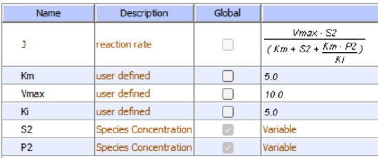
Let's look at an enzyme that converts reactant S to product P. Since P arises from S, they may have structural similarities. For example, what if GTP is the reactant and GDP the product? If so, then P might also bind in the active site and inhibit the conversion of S to P. This is called product inhibition. It probably occurs in most enzymes, and when it does, it will begin bending downward at the beginning of the progress curve for P formation. If the product binds very tightly, it may lead to a significant underestimation of the enzyme's initial velocity (v0) or flux (J0). Let's use Vcell to explore product inhibition. The model will explore two reactions:

• E + R ↔ ER → E + Q (no product inhibition)
• E + S ↔ ES → E + P (with product inhibition)

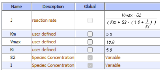
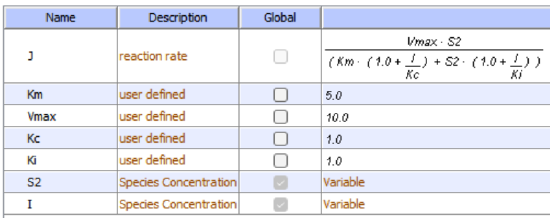
The chemical equation above does not explicitly show the product P binding the enzyme to form an EP complex. An actual reaction diagram showing the inhibition of an enzyme by an inhibitor I and by the product P is shown in Figure \(\PageIndex{6}\) below.

Figure \(\PageIndex{6}\): reaction diagram showing inhibition of an enzyme by an inhibitor I and by the product P

Vcell uses much simpler diagrams because it is most often used to model entire pathways or even entire cells. In simpler Vcell reaction diagrams, the inhibitor is typically not shown, since inhibition is built into the equation for the enzyme, represented by the node or yellow square in the figure above.

Let's now explore product inhibition in Vcell. In the reaction without product inhibition, R and Q are the reactant and product, respectively. S and P are used for the reaction with product P inhibition.

---

MODEL

Irreversible MM Kinetics - Without (left rx 1) and With (right, rx 2) Product Inhibition

Initial Conditions:  No product inhibition

Initial Conditions: With product inhibition

Select Load [model name] below

 Select Start to begin the simulation.

Interactive Element

Select Plot to change Y axis min/max, then Reset and Play  |  Select Slider to change which constants are displayed |  Select About  for software information.

Move the sliders to change the constants and see changes in the displayed graph in real-time.

Time course model made using Virtual Cell (Vcell), The Center for Cell Analysis & Modeling, at UConn Health.  Funded by NIH/NIGMS (R24 GM137787); Web simulation software (miniSidewinder) from Bartholomew Jardine and Herbert M. Sauro, University of Washington.  Funded by NIH/NIGMS (RO1-GM123032-04)

---

 

Inhibition by a competing substrate - the specificity constant

In the previous chapter, the specificity constant was defined as k_cat/K_M, which we also described as the second-order rate constant associated with the bimolecular reaction of E and S when S << K_M. It also describes how well an enzyme distinguishes between substrates. If an enzyme encounters two different substrates, one can be considered a competitive inhibitor of the other. The following equation gives the ratio of initial velocities for two competing substrates at the same concentration equal to the ratio of their k_cat/K_M values.

\begin{equation}
\frac{\mathrm{v}_{\mathrm{A}}}{\mathrm{v}_{\mathrm{B}}}=\frac{\frac{\mathrm{k}_{\mathrm{catA}}}{\mathrm{K}_{\mathrm{A}}} \mathrm{A}}{\frac{\mathrm{k}_{\mathrm{cat} \mathrm{B}}}{\mathrm{K}_{\mathrm{B}}} \mathrm{B}}
\end{equation}

A derivation of the specificity constant for an enzyme with competing substrates

Here it is!

Derivation

\begin{equation}
\mathrm{v}_{\mathrm{A}}=\frac{\mathrm{V}_{\mathrm{A}} \mathrm{A}}{\mathrm{K}_{\mathrm{A}}\left(1+\frac{\mathrm{B}}{\mathrm{K}_{\mathrm{B}}}\right)+\mathrm{A}} \quad \mathrm{v}_{\mathrm{B}}=\frac{\mathrm{V}_{\mathrm{B}} \mathrm{B}}{\mathrm{K}_{\mathrm{B}}\left(1+\frac{\mathrm{A}}{\mathrm{K}_{\mathrm{A}}}\right)+\mathrm{B}}
\end{equation}

\begin{equation}
\frac{\mathrm{v}_{\mathrm{A}}}{\mathrm{v}_{\mathrm{B}}}=\frac{\frac{\mathrm{V}_{\mathrm{A}} \mathrm{A}}{\mathrm{K}_{\mathrm{A}}\left(1+\frac{\mathrm{B}}{\mathrm{K}_{\mathrm{B}}}\right)+\mathrm{A}}}{\frac{\mathrm{V}_{\mathrm{B}} \mathrm{B}}{\mathrm{K}_{\mathrm{B}}\left(1+\frac{\mathrm{A}}{\mathrm{K}_{\mathrm{A}}}\right)+\mathrm{B}}}=\frac{\frac{\mathrm{V}_{\mathrm{A}} \mathrm{A}}{\mathrm{K}_{\mathrm{A}}+\frac{\mathrm{K}_{\mathrm{A}} \mathrm{B}}{\mathrm{K}_{\mathrm{B}}}+\mathrm{A}}}{\frac{\mathrm{V}_{\mathrm{B}} \mathrm{B}}{\mathrm{K}_{\mathrm{B}}+\frac{\mathrm{K}_{\mathrm{B}} \mathrm{A}}{\mathrm{K}_{\mathrm{A}}}+\mathrm{B}}}
\end{equation}

Now, in the above equation:

multiple the top half of the right-hand expression by \begin{equation}
\frac{\frac{1}{K_A}}{\frac{1}{K_A}}
\end{equation} multiple the bottom half of the right-hand expression by \begin{equation}
\frac{\frac{1}{K_B}}{\frac{1}{K_B}}
\end{equation} replace V_A with k_catAE₀ and V_B with k_catBE₀

This gives the following expression for v_A/v_B:

\begin{equation}
\frac{\mathrm{v}_{\mathrm{A}}}{\mathrm{v}_{\mathrm{B}}}=\frac{\frac{\mathrm{k}_{\mathrm{catA}}}{\mathrm{K}_{\mathrm{A}}} \mathrm{A}}{\frac{\mathrm{k}_{\mathrm{cat} \mathrm{B}}}{\mathrm{K}_{\mathrm{B}}} \mathrm{B}}
\end{equation}

Uncompetitive Inhibition

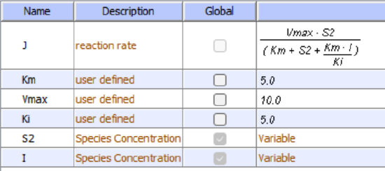
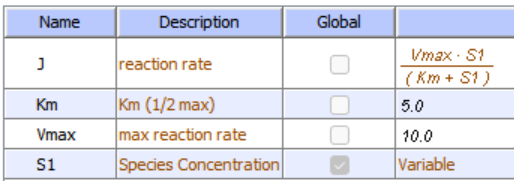
Reversible uncompetitive inhibition occurs when I binds only to ES and not free E. One can hypothesize that on binding S, a conformational change in E occurs, which presents a binding site for I. Inhibition occurs since ESI can not form the product. It is a dead-end complex that has only one fate: to return to ES. This is illustrated in the chemical equations and molecular cartoon shown in Figure \(\PageIndex{7}\).

Figure \(\PageIndex{7}\): Uncompetitive Inhibition

\begin{equation}
v_0=\frac{V_M S}{K_M+S\left(1+\frac{I}{K i i}\right)}=\frac{\left(\frac{V_M}{1+\frac{I}{K i i}}\right) S}{\left(\frac{K_M}{1+\frac{I}{K i i}}\right)+S}
\end{equation}

Let us assume that I binds reversibly to ES with a dissociation constant K_ii. The second "i" in the subscript "ii" indicates that the intercept of the 1/v vs 1/S Lineweaver-Burk plot changes while the slope stays constant. K_ii is also called K_iu, where the subscript "u" denotes the uncompetitive inhibition constant.

A look at the top mechanism shows that in the presence of I, as S increases to infinity, not all of E is converted to ES. There is a finite amount of ESI, even at an infinite S. Now remember that V_m = k_catE₀ if and only if all E is in the form ES. Under these conditions, the apparent V_m, V_mapp, is less than the true V_m without the inhibitor. In addition, the apparent K_m, K_mapp, will change. We can use LaChatelier's principle to understand this. If I binds to ES alone, and not E, it will shift the equilibrium of E + S ↔ ES to the right, which would have the effect of decreasing the K_mapp (i.e., it would appear that the affinity of E and S has increased). The double-reciprocal plot (Lineweaver-Burk plot) is a powerful way to visualize inhibition. In the presence of I, both V_m and K_m decrease. Therefore, -1/K_m, the x-intercept on the plot, will get more negative, and 1/V_m will get more positive. It turns out that they change to the same extent. Therefore, the plots will consist of a series of parallel lines, which is the hallmark of uncompetitive inhibition, as shown in Figure \(\PageIndex{8}\).

Figure \(\PageIndex{8}\): Uncompetitive Inhibition: Lineweaver-Burk plots

Here is an interactive graph showing v₀ vs [S] for uncompetitive inhibition with Vm and Km both set to 100. Change the sliders for [I] and Kis and see the effect on the graph.

Here is an interactive graph showing uncompetitive inhibition with Vm and Km both set to 10. Change the sliders for [I] and Kii and see the effect on the graph

An equation shown in the diagram above can be derived to describe the effect of the uncompetitive inhibitor on the reaction velocity. The only change is that the S term in the denominator is multiplied by the factor 1+I/Kii. We want to rearrange this equation to show how K_m and V_m are affected by the inhibitor, not S. Rearranging the equation above yields K_mapp = K_m/(1 + I/K_ii) and V_mapp = V_m/(1 + I/K_ii). This shows that the apparent Km and Vm do decrease as we predicted. Kii is the inhibitor dissociation constant, in which the inhibitor affects the intercept of the double-reciprocal plot. Note that if I = 0, K_m and V_m remain unchanged.

Progress Curves: Uncompetitive Inhibition

Now, let's compare the progress curves for an enzyme-catalyzed reaction in the absence and presence of an uncompetitive inhibitor.

---

MODEL

No inhibition (left) and Uncompetitive Inhibition (right)

(Note the the Vcell reaction diagram is the same as for competitive inhibition.  However, the mathematical equations differ as shown below.

Initial values No Inhibition

Initial values With Uncompetitive Inhibitor

I is fixed for each simulation (as it is not converted to a product) but can be changed in the simulation below.

Select Load [model name] below

 Select Start to begin the simulation.

Interactive Element

Select Plot to change Y axis min/max, then Reset and Play  |  Select Slider to change which constants are displayed |  Select About  for software information.

Move the sliders to change the constants and see changes in the displayed graph in real-time.

Time course model made using Virtual Cell (Vcell), The Center for Cell Analysis & Modeling, at UConn Health.  Funded by NIH/NIGMS (R24 GM137787); Web simulation software (miniSidewinder) from Bartholomew Jardine and Herbert M. Sauro, University of Washington.  Funded by NIH/NIGMS (RO1-GM123032-04)

---

 

 

Figure \(\PageIndex{9}\) shows an interactive iCn3D model of an uncompetitive inhibitor of the cysteine protease caspase-6 (4HVA)

Figure \(\PageIndex{9}\):  Uncompetitive inhibitor of the cysteine protease caspase-6 (4HVA) . (Copyright; author via source).
Click the image for a popup or use this external link: https://structure.ncbi.nlm.nih.gov/i...TVfKio7NxcpX28

The "substrate" in this model (cyan, transparent surface, with labels on V, E, and I) is a substrate analog, VEI-CHO, in which the tripeptide substrate VEI ends not in a free carboxyl or amide group but in an aldehyde, which causes this "substrate" to become covalently attached to the enzyme and act as an inhibitor.  The uncompetitive inhibitor (gray, transparent surface) binds to the blue surface.  Hence, it binds to the ES complex.  Two active site residues, Cys 163, the active site nucleophile, and His 121, a catalytic acid/base, are shown in colored sticks and labeled.

Figure \(\PageIndex{10}\) below shows a Lineweaver-Burk plot showing 1/v_o vs 1/[S], where the substrate is the divalent compound (VEID)₂R110.    Its N-terminus is capped with a benzyloxy (Z) group.  R110 is a rhodamine-type fluorophore, which, on cleavage, gives a strong fluorescent signal that the benzyloxy group initially quenches in the uncleaved substrate.

Figure \(\PageIndex{10}\): Double-reciprocal Lineweaver-Burk plot of compound 3 with (VEID)₂R110 substrate showing uncompetitive inhibition.  Heise CE et al. (2012) Mechanistic and Structural Understanding of Uncompetitive Inhibitors of Caspase-6. PLoS ONE 7(12): e50864. https://doi.org/10.1371/journal.pone.0050864.  Creative Commons Attribution License.

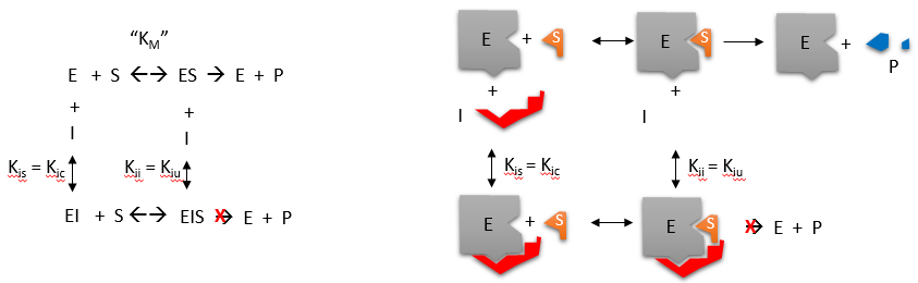
Noncompetitive and Mixed Inhibition

Reversible noncompetitive inhibition occurs when I binds to both E and ES. We will look at only the special case in which the dissociation constants of I for E and ES are the same. This is called noncompetitive inhibition. It is quite rare, as it would be difficult to imagine a large inhibitor that inhibits the turnover of a bound substrate and does not affect the binding of S to E. However, the covalent interaction of protons with both E and ES can lead to noncompetitive inhibition. In the more general case, the Kd's are different, and the inhibition is called mixed. Since inhibition occurs, we will hypothesize that ESI can not form the product. It is a dead-end complex with only one fate: to return to ES or EI. This is illustrated in the chemical equations and the molecular cartoon in Figure \(\PageIndex{11}\).

Figure \(\PageIndex{11}\): Noncompetitive and Mixed Inhibition

Let us assume for ease of equation derivation that I binds reversibly to E with a dissociation constant of K_is (as we denoted for competitive inhibition) and to ES with a dissociation constant K_ii (as we noted for uncompetitive inhibition). Assume that for noncompetitive inhibition, K_is = K_ii. A look at the top mechanism shows that in the presence of I, as S increases to infinity, not all of E is converted to ES. There is a finite amount of ESI, even at infinite S. Now remember that V_m = k_catE₀ if and only if all E is in the form ES. Under these conditions, the apparent V_m, V_mapp, is less than the real Vm without an inhibitor. In contrast, the apparent K_m, K_mapp, will not change since I binds to both E and ES with the same affinity and hence will not perturb that equilibrium, as deduced from LaChatelier's principle. The double-reciprocal plot (Lineweaver-Burk plot) is a powerful way to visualize inhibition. In the presence of I, just V_m will decrease. Therefore, -1/K_m, the x-intercept will stay the same, and 1/V_m will become more positive. Therefore, the plots will consist of a series of lines intersecting on the x-axis, the hallmark of noncompetitive inhibition. You should be able to figure out how the plots would look if K_is differs from K_ii (mixed inhibition).

\begin{equation}
v_0=\frac{V_M S}{K_M\left(1+\frac{I}{K i s}\right)+S\left(1+\frac{I}{K i i}\right)}
\end{equation}

The equation shown in the diagram above can be derived to describe the effect of a noncompetitive inhibitor on reaction velocity. Km is multiplied by 1+I/K_is, and S by 1+I/K_ii in the denominator. We want to rearrange this equation to show how the inhibitor affects Km and Vm, not S. Rearranging the equation as shown above shows that K_mapp = K_m(1+I/K_is)/(1+I/K_ii) = K_m when K_is = K_ii, and V_mapp = V_m/(1+I/K_ii). This shows that K_m remains unchanged and that V_m decreases as we predicted. The plot shows a series of lines intersecting on the x-axis as shown in Figure \(\PageIndex{12}\). Both the slope and the y-intercept are changed, which are reflected in the names of the two dissociation constants, K_is and K_ii. Note that if I is zero, K_mapp = K_m and V_mapp = V_m. Sometimes, the K_is and K_ii inhibition dissociation constants are called K_c and K_u (competitive and uncompetitive inhibition dissociation constants.

Figure \(\PageIndex{12}\): Noncompetitive Inhibition: Lineweaver-Burk plots

Move the sliders on this interactive graph below to show how changes in K_is and K_ii affect the position on the graph where the lines intersect. Try changing their values to shift the graph intersections from the top-left quadrant to the bottom-left quadrant.

Here is an interactive graph showing v₀ vs [S] for mixed inhibition with Vm and Km both set to 100. Change the sliders for [I] and Kis and see the effect on the graph

Here is an interactive graph showing mixed inhibition with Vm and Km both set to 10. Change the sliders for [I] and Kii and see the effect on the graph

Progress Curves: Mixed/Noncompetitive Inhibition

Now let's compare the progress curves for an enzyme-catalyzed reaction in the absence and presence of a mixed inhibitor.

---

MODEL

No inhibition (left) and Uncompetitive Inhibition (right)

Note that the Vcell reaction diagram is the same as for competitive and uncompetive inhibition.  It doesn't explicitly show that the mixed inhibitor binds to both free and substrate-bound enzymes.  Those interactions are addressed in the mathematical equations for mixed inhibition.

Initial values No Inhibition

Initial values With Uncompetitive Inhibitor

I is fixed for each simulation (as it is not converted to a product) but can be changed in the simulation below.

Select Load [model name] below

 Select Start to begin the simulation.

Interactive Element

Select Plot to change Y axis min/max, then Reset and Play  |  Select Slider to change which constants are displayed |  Select About  for software information.

Move the sliders to change the constants and see changes in the displayed graph in real-time.

Time course model made using Virtual Cell (Vcell), The Center for Cell Analysis & Modeling, at UConn Health.  Funded by NIH/NIGMS (R24 GM137787); Web simulation software (miniSidewinder) from Bartholomew Jardine and Herbert M. Sauro, University of Washington.  Funded by NIH/NIGMS (RO1-GM123032-04)

---

 

Mixed and noncompetitive inhibition (as shown by the mechanism above) differ from competitive and uncompetitive inhibition. Inhibitor binding is not simply a dead-end reaction in which the inhibitor can dissociate only in a single reverse step. In the above equilibrium, S can dissociate from ESI to form EI, so the system may not be at equilibrium. With dead-end steps, no flux of reactants occurs through the dead-end complex, so the equilibrium for the dead-end step is not perturbed.

Other mechanisms can commonly give mixed inhibition. For example, the product released in a ping pong mechanism (discussed in the next chapter) can give mixed inhibition. A ping pong reaction mechanism is shown and superficially explained in Figure \(\PageIndex{13}\).

Figure \(\PageIndex{13}\): Ping pong reaction mechanism

If P, acting as a product inhibitor, can bind to two different forms of the enzyme (E' and E), it will act as a mixed inhibitor.

Figure \(\PageIndex{14}\) shows an interactive iCn3D model of a noncompetitive inhibitor of M. tuberculosis's class IIa fructose 1,6-bisphosphate aldolase (4LV4).

Figure \(\PageIndex{14}\):  Noncompetitive inhibitor of M. tuberculosis's class IIa fructose 1,6-bisphosphate aldolase (4LV4). (Copyright; author via source).
Click the image for a popup or use this external link: https://structure.ncbi.nlm.nih.gov/i...wZDtkvtwqnrVy7

The non-competitive inhibitor, 8-hydroxyquinoline carboxylic acid (HCA), is shown in cyan.  Active-site side chains of the Zn²⁺-containing enzyme are shown as colored sticks, labeled.

The noncompetitive inhibitor does not enter into the pocket where the substrate (not shown in the model above) binds.  The binding of the noncompetitive inhibitor causes a conformational change that moves the Zn-binding loop (Z-loop), which contains His 212, which coordinates the Zn²⁺ ion.  Hence, the Zn-loop is part of the active site, and when it moves upon inhibitor binding, access to the empty pocket where the substrate binds is hindered.   When Zn²⁺ moves away from the active site, it can no longer catalyze the reaction. 

Enzyme Inhibition in Vivo

The pharmaceutical industry is devoted to finding drug molecules that affect biological processes. Typically, this means developing small-molecule inhibitors for target proteins. Recent work has expanded to include the development of inhibitory RNA molecules that affect DNA transcription and mRNA translation. Using combinatorial synthetic techniques and computational modeling, developing small-molecule inhibitors (especially competitive ones) that inhibit proteins in vitro using purified enzymes, substrates, and inhibitors in lab testing has become easier. Assuming that the inhibitor could pass through the membrane and accumulate to a sufficient concentration, would it have the same inhibitory properties in the cell as in the test tube? The answer turns out to be maybe. Remember that a cell is tightly packed with a multitude of other small molecules and macromolecules. In addition, the enzyme targeted for inhibition is most likely part of a pathway of enzymes that feed reactants into the enzyme and remove the product. Hence, the flux of substrate and product is controlled by the entire pathway and not just the single target enzyme. The target enzyme's product concentration is determined by the enzyme's kinetic parameters and the available substrate concentration.

The conditions under which enzymes are studied (in vitro) and those under which they operate (in vivo) are very different.

• In vitro (in the lab), the enzyme is held at a constant concentration while the substrate is varied (i.e., the substrate concentration is the independent variable). The velocity is determined by the substrate concentration. When inhibition is studied, the substrate is varied while the inhibitor is held constant at several different fixed concentrations.
• In vivo (in the cell), the velocity might be relatively fixed, with the substrate concentration determined by the velocity. The substrate can't build up at the enzyme to avoid a flux bottleneck, so the enzyme processes it in a steady-state manner to produce the product, as determined by the Michael-Menten equation.

What happens when an inhibitor is added in vivo? Let's assume that the enzyme is running at v = V_m/2. How might in vivo inhibition plots look at constant velocity (for example, v=V_m/2) when both I and S can vary, and in which S for an enzyme in the middle of a pathway is determined by v?

The equations and graph below show the ratio of S/K_m vs I/K_ix for inhibition at constant v, a condition encountered when an enzyme in a metabolic pathway is subject to flux controls imposed by the entire pathway. The x-axis reflects the ratio of inhibitor concentration to its inhibition constant. Likewise, the y-axis reflects the relative amount of substrate compared to its K_m. The graph for in vivo competitive inhibition is linear, but it "blows up" for uncompetitive inhibition, as shown in Figure \(\PageIndex{15}\).

Figure \(\PageIndex{15}\): S/K_m vs 1/K_ix plots for competitive and uncompetitive inhibition

Here are the derivations used to produce the graphs in Figure \(\PageIndex{13}\).

A derivation of the competitive and uncompetitive inhibition in vivo when v = constant

Here it is!

Derivation

Competitive Inhibition at constant velocity v:

Let's start with the equation of competitive inhibition.

\begin{equation}
\mathrm{v}=\frac{\mathrm{V}_{\mathrm{M}} \mathrm{S}}{\mathrm{K}_{\mathrm{M}}\left(1+\frac{\mathrm{I}}{\mathrm{K}_{\mathrm{is}}}\right)+\mathrm{S}}
\end{equation}

Let

\begin{equation}
\left(1+\frac{\mathrm{I}}{\mathrm{K}_{\mathrm{is}}}\right)=\mathrm{y}
\end{equation}

Then,

\begin{equation}
\begin{gathered}
v=\frac{V_M S}{K_M y+S} \\
v\left(K_M y+S\right)=V_M S \\
v K_M y+v S=V_M S \\
v K_M y=V_M S-v S=S\left(V_M-v\right) \\
K_M=\frac{S\left(V_M-v\right)}{v y}
\end{gathered}
\end{equation}

which gives:

\begin{equation}
\begin{gathered}
\frac{S}{K_M}=\frac{v y}{\left(V_M-v\right)}=\frac{y}{\frac{V_M}{v}-1}=\frac{1+\frac{I}{K_{i s}}}{\frac{V_M}{v}-1}=\frac{1}{\frac{V_M}{v}-1}+\frac{\frac{I}{K_{i s}}}{\frac{V_M}{v}-1} \\
\frac{S}{K_M}=\frac{1}{\frac{V_M}{v}-1}+\left(\frac{1}{\frac{V_M}{v}-1}\right) \frac{I}{K_{i s}}
\end{gathered}
\end{equation}

Note from the last equation that the graph of S/K_M vs I/K_is is linear (at a fixed v), as shown in the above figure.

Uncompetitive Inhibition at constant velocity v:

Let's start with the equation of uncompetitive inhibition.

\begin{equation}
\mathrm{v}=\frac{\mathrm{V}_{\mathrm{M}} \mathrm{S}}{\mathrm{K}_{\mathrm{M}}+\mathrm{S}\left(1+\frac{\mathrm{I}}{\mathrm{K}_{\mathrm{ii}}}\right)}
\end{equation}

Let

\begin{equation}
\left(1+\frac{1}{\mathrm{K}_{\mathrm{ii}}}\right)=\mathrm{y}
\end{equation}

then:

\begin{equation}
\begin{gathered}
v=\frac{V_M S}{K_M+S y} \\
v\left(K_M+S y\right)=V_M S \\
v K_M=V_M S-v S y=S\left(V_M-v y\right)
\end{gathered}
\end{equation}

which gives:

\begin{equation}
\frac{S}{K_M}=\frac{v}{V_M-v y}\left(\frac{\frac{1}{v}}{\frac{1}{v}}\right)=\frac{1}{\frac{V_M}{v}-y}=\frac{1}{v-1-\frac{I}{K_{i i}}}
\end{equation}

This graph is not a linear function of I/K_ii as it was for in vivo competitive inhibition.

• for competitive inhibition, the graph of S/K_M is a linear function of I/K_is
• for uncompetitive inhibition, the graph of S/K_M is NOT a linear function of I/K_ii but rather "blows up" to infinity.

These graphs and associated equations are dramatically different from the very similar forms of inhibition equations and curves for in vitro inhibition at varying S and different fixed values of inhibitor. Consider the uncompetitive graph and equation. In the absence of an inhibitor, if S=Km, then Vm/v = 2, so the calculated value from the equation above of S/Km = 1. The y-intercept of the graph above is 1 for uncompetitive (and competitive) inhibition. If I is allowed to increase to a value of Kii (so I/Kii = 1), again at constant v=Vm/2, then the right-hand side goes to infinity.

In a linked series of reactions, if the middle reaction is inhibited, the substrate for that enzyme builds, whether the inhibition is competitive or uncompetitive. In competitive inhibition, the substrate concentration can be increased to meet the enzyme's requirements. However, as the above figure shows, this can't happen with uncompetitive inhibition, since as more substrate accumulates, the reaction reaches a point at which steady state is lost.

Obviously, this limiting case can't be realistically reached, but it does suggest that uncompetitive inhibitors would be more effective in vivo in controlling a metabolic pathway than competitive inhibitors. Cornish-Bowden argues that purely uncompetitive inhibitors are rare because of the degree of inhibition they can hypothetically produce (1986). Likewise, he suggests that medicinal chemists should synthesize uncompetitive inhibitors if their goal is to maximally inhibit a metabolic pathway under the kind of flux control described above. Although it is more difficult to synthesize a purely uncompetitive inhibitor, as it can't be easily modeled after the structure of a natural ligand that binds to the active site than competitive inhibitors, he notes that synthesizing mixed (and noncompetitive) inhibitors whose Kii values are of reasonable size compared to their Kis values, would be one approach.

Move the sliders on the interactive graph below to show how the graphs change. Disregard the graph in the right lower quadrant, as that location would require negative values of either S or K.

Inhibition by Temperature and pH Changes

From 0 to about 40-50 ^oC, enzyme activity usually increases, as do the rates of most reactions in the absence of catalysts. (Remember the general rule of thumb that reaction velocities double for each increase of 10 ^oC). At higher temperatures, the enzyme's activity decreases dramatically as it denatures. These features are illustrated in Figure \(\PageIndex{16}\).

Figure \(\PageIndex{16}\): Temperature effects on enzyme activity

Likewise, pH has a marked effect on the velocity of enzyme-catalyzed reactions as illustrated in Figure \(\PageIndex{17}\).

Figure \(\PageIndex{17}\): pH effects on enzyme activity

Think of all the things that pH changes might affect. It might

• affect E in ways to alter the binding of S to E, which would affect K_m
• affect E in ways to alter the actual catalysis of bound S, which would affect k_cat
• affect E by globally changing the conformation of the protein
• affect S by altering the protonation state of the substrate

The easiest assumption is that key side chains necessary for catalysis must be in the correct protonation state. Thus, a sidechain, with an apparent pKa of around 6, must be deprotonated for optimal trypsin activity, which shows a pH-dependent increase centered at pH 6. Which amino acid side chain would be a likely candidate?

Table \(\PageIndex{1}\) below shows how pH effects on enzyme kinetics can be modeled at the chemical and mathematical level.

\begin{equation} \begin{gathered} \mathrm{v}_{0}=\frac{\mathrm{V}_{\mathrm{m} \mathrm{app}} \mathrm{S}}{\mathrm{K}_{\mathrm{m}} \text { app }}+\mathrm{S} \\ \mathrm{V}_{\mathrm{m} \text { app }}=\frac{\mathrm{V}_{\mathrm{m}}}{1+\frac{\mathrm{H}^{+}}{\mathrm{K}_{\mathrm{ES} 1}}+\frac{\mathrm{K}_{\mathrm{ES} 2}}{\mathrm{H}^{+}}} \\ \mathrm{K}_{\mathrm{m} \text { app }}=\frac{\mathrm{K}_{\mathrm{m}}\left(1+\frac{\mathrm{H}^{+}}{\mathrm{K}_{\mathrm{ES} 1}}+\frac{\mathrm{K}_{\mathrm{ES} 2}}{\mathrm{H}^{+}}\right)}{1+\frac{\mathrm{H}^{+}}{\mathrm{K}_{\mathrm{ES} 1}}+\frac{\mathrm{K}_{\mathrm{ES} 2}}{\mathrm{H}^{+}}} \end{gathered} \end{equation}

 

Summary

(Summary written by Claude, Sonnet 4.6, Anthropic)

This chapter develops the quantitative framework for enzyme inhibition — the reduction of catalytic activity by molecules that bind to the enzyme — covering the major reversible inhibition mechanisms, their mathematical descriptions, their Lineweaver-Burk signatures, special cases including product inhibition and substrate competition, and the physiologically important differences between inhibition analyzed in vitro versus in vivo.

Irreversible covalent inhibition provides a conceptual baseline: reagents that chemically modify essential active site residues (for example, iodoacetamide, which alkylates a catalytic Cys) permanently inactivate the enzyme. Distinguishing which residue is critical requires protection experiments in which a saturating ligand occupies the active site during chemical modification, with the extent of protection depending on KD and ligand concentration. However, the majority of pharmacologically relevant inhibition is reversible and noncovalent.

Competitive inhibition occurs when inhibitor I and substrate S compete for the same binding site on free enzyme E, binding in a mutually exclusive fashion (either through direct overlap of binding sites or through allosteric conformational changes that make one site inaccessible when the other is occupied). The key kinetic consequences follow from Le Chatelier's principle: I binding to free E shifts the E + S ↔ ES equilibrium leftward, increasing the apparent K_M. However, at infinite [S], all E is driven into the ES form regardless of I concentration, so V_M is unchanged. The modified velocity equation v₀ = V_M[S]/(K_M(1 + I/K_IS) + [S]) shows that K_Mapp = K_M(1 + I/K_IS) grows with increasing I while V_M is unaffected. On Lineweaver-Burk plots, competitive inhibition produces a family of lines with the same y-intercept (1/V_M) but progressively more positive slopes (K_M(1 + I/K_IS)/V_M) and x-intercepts moving toward zero (−1/K_Mapp). Competitive inhibitors are typically substrate analogs that mimic the structure of S, as illustrated by the buffer component MES, which acts as a competitive inhibitor of phosphotyrosyl phosphatase by mimicking the phosphate group of phosphotyrosine substrates.

Uncompetitive inhibition occurs when I binds only to the ES complex, not to free E — perhaps because substrate binding induces a conformational change that creates the inhibitor binding site. Since I cannot bind free E, it cannot compete with S for E; instead, it traps ES in a dead-end ESI complex. By Le Chatelier's principle, I binding to ES shifts the E + S ↔ ES equilibrium rightward, which paradoxically decreases K_Mapp = KM/(1 + I/K_ii) while also decreasing V_Mapp = V_M/(1 + I/K_ii) — both change by the same factor (1 + I/K_ii). On Lineweaver-Burk plots, this produces the hallmark of uncompetitive inhibition: a family of parallel lines (constant slope K_M/V_,, but shifted intercepts), distinguishing it from competitive inhibition where lines converge on the y-axis.

Noncompetitive inhibition is a special case of mixed inhibition in which I binds to both E and ES with equal dissociation constants K_IS = K_ii. Since I binds both forms equally, it does not perturb the E + S ↔ ES equilibrium, and K_M is unchanged. However, since ESI is a dead-end complex that cannot produce product, V_Mapp = V_M/(1 + I/K_ii) is reduced. On Lineweaver-Burk plots, noncompetitive inhibition gives lines with a common x-intercept (−1/KM, since KM is unchanged) but increasing y-intercepts (1/VMapp), distinguishing it from competitive and uncompetitive cases. In mixed inhibition (the more general case where K_IS ≠ K_ii), both K_Mapp = K_M(1 + I/K_IS)/(1 + I/K_ii) and V_Mapp = V_M/(1 + I/K_ii) change, and Lineweaver-Burk lines intersect in a quadrant displaced from either axis. The specificity constant k_cat/K_M governs competition between substrates: when two substrates compete for the same active site, the ratio of their initial velocities at equal concentration equals the ratio of their k_cat/K_M values, explaining how an enzyme discriminates among substrates in vivo.

Product inhibition — a special case of competitive inhibition in which the structurally similar product P occupies the active site — occurs in most enzymes to some degree and causes downward curvature in P vs. t progress curves as product accumulates. Tight product binding can significantly underestimate measured v₀ if initial rates are not determined carefully. The ping-pong reaction mechanism (two-substrate, two-product reactions with a covalent intermediate) can also generate mixed inhibition when the released product can bind to two different enzyme forms.

The physiological significance of inhibitor type is dramatically revealed by in vivo analysis. In the test tube, [S] is the independent variable and [I] is held constant. In the cell, however, an enzyme embedded in a metabolic pathway operates under approximately constant flux v, and [S] adjusts to satisfy the Michaelis-Menten equation rather than being experimentally controlled. Under constant flux conditions, deriving S/K_M as a function of I/K_IS (competitive) or I/K_ii (uncompetitive) reveals a striking difference: competitive inhibition gives a linear S/K_M vs. I/K_IS relationship (the substrate concentration rises proportionally to compensate for the inhibitor), while uncompetitive inhibition makes S/K_M go to infinity as I → K_ii — meaning that no amount of substrate buildup can restore the required flux. This analysis, originally articulated by Cornish-Bowden, implies that uncompetitive inhibitors (and mixed inhibitors with relatively small K_ii compared to K_IS) would be far more effective at disrupting metabolic pathways in vivo than competitive inhibitors — a counterintuitive conclusion with important implications for drug design, since competitive inhibitors are most commonly developed due to their structural similarity to natural substrates.

Finally, pH affects enzyme activity by altering the protonation state of catalytically essential residues — typically requiring specific protonation states for general acid/base catalysis (affecting kcat) or for electrostatic interactions that position the substrate (affecting K_M) — and produces characteristic bell-shaped activity-pH profiles whose inflection points reflect the apparent pKa values of critical active site residues. Temperature increases enzyme activity up to ~40–50°C via standard Arrhenius kinetics but causes a precipitous drop in activity above this range as the protein denatures, reflecting the thermodynamic marginal stability of folded proteins discussed in earlier chapters.