6.2: Kinetics without Enzymes

Search Fundamentals of Biochemistry

Learning Goals (ChatGPT o1, 1/30/25)

(Learning goals written by Claude, Sonnet 4.6, Anthropic)

Single-Step Reaction Kinetics

• Understand the use of calculus in describing reaction kinetics, including the meaning of the derivative dX/dt as the instantaneous rate of change in concentration and translate between the differential (dX/dt) and integrated (X as a function of time) forms of rate equations
• Distinguish initial rate analysis (measuring v₀ as the initial slope of a concentration vs. time curve at approximately constant [A] = A₀) from integrated rate analysis (fitting the full progress curve [A] = f(t) to the solution of the differential equation), and explain when each approach is experimentally advantageous.
• Write and interpret the differential equation for a first-order reaction (d[A]/dt = −k₁[A]), derive or recognize the integrated solution [A] = [A₀]e^(−k₁t), and use the diagnostic graphical tests — exponential decay of [A] vs. t and linearity of ln[A] vs. t with slope −k₁ — to confirm first-order behavior from experimental data.
• Write and interpret the differential equation for a second-order reaction (d[A]/dt = −k₂[A]²), recognize the integrated solution that predicts a linear rise in 1/[A] vs. t with slope k₂, explain the concept of pseudo-first-order conditions when [B] >> [A] (giving an apparent first-order rate constant k₁' = k₂[B]), and explain why second-order reactions are faster than first-order reactions at high [A] but slower at low [A].

Multi-Step Reaction Kinetics

• Write the coupled differential equations for the reversible first-order reaction A ↔ P (d[A]/dt = −k₁[A] + k₋₁[P] and d[P]/dt = k₁[A] − k₋₁[P]), interpret the progress curves showing how the plateau concentrations of A and P depend on the ratio k₁/k₋₁, and connect this ratio to the equilibrium constant Keq = k₁/k₋₁ = [P]eq/[A]eq — recognizing that at equilibrium, forward and reverse fluxes are equal but nonzero.
• Write the differential equations for consecutive irreversible reactions A → B → C, describe qualitatively how the shape of the B vs. t progress curve (a transient intermediate that rises then falls) depends on the relative magnitudes of k₁ and k₂, and explain why the time to maximum [B] and the degree of accumulation of B are determined by whether k₁ >> k₂ or k₂ >> k₁.
• Explain how numerical simulation tools such as VCell and COPASI, which implement Systems Biology Markup Language (SBML) models, make it practical to obtain progress curves for fully reversible multi-step reactions (A ↔ B ↔ C) whose analytical solutions are intractable — and describe how interactive sliders changing rate constants (k₁f, k₁r, k₂f, k₂r) allow exploration of how each rate constant individually influences the time-dependent concentrations of all species.

 

Single Step Reactions

First, we will explore the kinetics of non-catalyzed reactions, which is needed to understand the kinetics of the more complicated enzyme-catalyzed reactions.

Calculus: Derivatives and Integrals

In this book, we will refer to the change of concentration of a chemical species X as a function of time as dX/dt instead of ΔX/Δt, where dX/dt is the derivative of X with respect to time t. This is the language of calculus, which most readers would have studied. The use of calculus will be mainly limited to writing equations of the form dX/dt = f(t), a type of differential equation. We will also use a few integrals, but a working knowledge of calculus is not required. For readers who have not studied calculus, replace dX/dt with ΔX/Δt in your mind, and you will derive the same meaning.

You studied two types of kinetic equations in introductory chemistry to analyze kinetic data:

• Initial Rates: In this method, the initial rate, v₀, is measured as a function of the concentration of reactants. The initial velocity, v₀, is the initial slope of a graph of the concentration of reactants or products as a function of time, taken over a range of times such that only a small fraction of A has reacted. Under this condition, [A] over this short time range is approximately constant and equal to Ao. Initial rate graphs are often based on the measurement of product increase with time, ΔP/Δt, so v₀ vs. A plots have positive slopes. The velocity at time t along the A vs. t curve, dA/dt, constantly changes as [A] decreases since the velocity depends on [A]. To reiterate, the initial velocity of the reaction is the slope of the initial linear part of the decay curve when the rate is essentially linear over a narrow range of [A].
• Integrated Rates and Progress Curves: In this method, a differential equation that gives the change of A or P with time (dA/dt or dP/dt) is integrated to give an equation that shows the concentration of A or P as a function of time. For any given reaction, it is essential to be able to write the integrated rate equation, often called an ordinary differential equation (ODE). In almost every case, we provide the solutions to the ODEs in either a mathematical equation or a fitted graph of A vs. t. As the reactions get more complicated, we let computers solve them numerically and show the output. The ODEs are also called progress curves as they show how the concentration of reactants and products changes with time.

In either case, the mathematical equations describing the reaction are used to fit experimental data taken in the lab. Statistics are used to see how closely the experimental data fit the rate equations. The best-fit equation gives the most likely chemical reaction equations for the interconversion of reactants and products.

Most biochemistry textbooks focus on initial velocities when explaining enzyme kinetics. However, in many ways, this method is less intuitive than exploring how the concentration of a molecule changes with time. An analogy is the concept of density (mass/volume), which is more complicated than understanding mass or volume separately. We use both methods to develop both chemical and biological intuitions of kinetic properties.

We will first explore simple irreversible reactions (1^st and 2^nd order), then make them reversible, and then couple them together to form more complex reaction schemes, much as we are compelled to do for enzyme-catalyzed reactions.

First Order Reaction

\[\ce{A ->[k_{1}] P} \nonumber \]

where k₁ is the first-order rate constant. For these reactions, the velocity of the reaction, \(v\), is directly proportional to [A], or

\[v=-\frac{d A}{d t}=+\frac{d P}{d t}=k_{1} A \label{6.3.A.1} \]

The negative sign in -d[A]/dt indicates that the concentration of A decreases. The equation could also be written as:\(v=\frac{d A}{d t}=-k_{1} A\)

For the rest of the reactions in this book, we follow the convention of writing all velocities expressed as d[x]/dt as positive numbers. A negative sign for a term on the right-hand side of the differential equation will indicate that the concentration dependency of that term will lead to a decrease in [x] with time. Likewise, a positive sign for the term on the right-hand side of the equation will indicate that the concentration dependency of that term will lead to an increase in [x] with time.

Examples: dA/dt = -kA shows that A will decrease with time. dA/dt = +kA shows that A will increase with time.

Here is the solution to the differential Equation 6.3.A.1 for [A] as a function of t.

\begin{equation}
A=A_0 e^{-k_1 t}
\end{equation}

A derivation of the first order rate equation

Here it is!

Derivation

\begin{equation}
\begin{gathered}
\int_{A_O}^A \frac{d A}{A}=-k_1 \int_0^t d t \\
\ln A-\ln A_0=-k_1 t \\
\ln A=\ln A_0-k_1 t \\
A=A_0 e^{-k_1 t}
\end{gathered}
\end{equation}

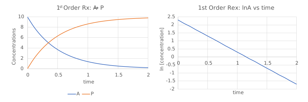
Equation 6.3.A.2 is an example of an integrated rate equation. The following graphs show plots of A vs t and lnA vs. t for a first-order process. Note that the derivative of the graph of A vs. t (dA/dt) is the velocity of the reaction. The graph of ln[A] vs. t is linear with a slope of -k₁. The velocity of the reaction (slope of the A vs t curve) decreases with decreasing A, which is consistent with equation 1. Again, the initial velocity is determined from data taken in the first part of the decay curve when the rate is linear and little A has reacted. That is, [A] is approximately equal to [A₀].

Figure \(\PageIndex{1}\) shows two ways to plot 1^st order reaction data. The left graph shows the exponential decay of A with time and the corresponding rise in P when A₀ is 0 and k₁=2. The other shows the linear fall of ln[A] vs time.

Figure \(\PageIndex{1}\): Two ways to plot 1^st order reaction data

Once again, for complete clarification, another way of analyzing the kinetics of a reaction, in addition to following the concentration of a reactant or product as a function of time and fitting the data to an integrated rate equation, is to plot the initial velocity, vo, of the reaction as a function of the concentration of reactants. The initial velocity is the initial slope of a graph of the concentration of reactants or products as a function of time, taken over a range of times such that only a small fraction of A has reacted, so [A] is approximately constant = Ao. From the first-order graph of A vs. t above, the slope approaches 0 with increasing time as [A] approaches 0, which indicates that the reaction velocity depends on A. For this first-order process, two equivalent equations can be written showing the disappearance of A as v = -d[A]/dt = k1[A], while appearance of A as v = d[A]/dt = -k1[A], Both equations show that v is directly proportional to A. As [A] is doubled, the initial velocity is doubled. Velocity graphs used by biochemists often show the initial velocity of product formation (not reactant decrease) as a function of reactant concentration. Hence, as product concentration increases, the initial velocity is positive. A graph of v (= dP/dt) vs [A] for a first-order process would have a positive slope and be interpreted as showing that the rate of appearance of P depends linearly on [A].

Second-Order/Pseudo First-Order Reactions

\begin{equation}
A+B \stackrel{k_2}{\longrightarrow} P \text { or } A+A \stackrel{k_2}{\longrightarrow} P
\end{equation}

where \(k_2\) is the second-order rate constant. For the first of these irreversible reactions, the velocity of the reaction, v, is directly proportional to [A] and [B], or

\begin{equation}
v=\frac{d A}{d t}=-k_2[A][B]
\end{equation}

We will consider two special cases of this reaction type:

1. [B] >> [A]. Under these conditions, [B] never changes, so Equation 5 becomes

\begin{equation}
v=-\left(k_2[B]\right)[A]=-k_1^{\prime}[A]
\end{equation}

where k₁' is the pseudo first order rate constant (= k2[B] ) for the reaction. The reaction appears to be first order, depending only on [A].

2. As illustrated in the second reaction above, the only reactant is A, which must collide with another A to form P.

The following differential equation can be written and solved to find [A] as a function of t.

\begin{equation}
v=\frac{d A}{d t}=2 \frac{d P}{d t}=-k_2 A^2
\end{equation}

Solving the differential equation for A gives the following:

\begin{equation}
\frac{1}{A}=\frac{1}{A_0}+k_2 t
\end{equation}

A derivation of the second order rate equation

Here it is!

Derivation

\begin{equation}
\begin{gathered}
\frac{d A}{d t}=-k_2 A^2 \\
\int_{A_0}^A \frac{d A}{A^2}=\int_{A_0}^A A^{-2} d A=\int_{A_0}^A A^{-2} d A=-k_2 \int_0^t d t \\
\left.\left.\left.\frac{A^{n+1}}{n+1}\right]_{A_0}^A=\frac{A^{-1}}{-1}\right]_{A_0}^A=-k_2 t\right]_{A_0}^A \\
-\frac{1}{A}-\left(\frac{1}{A_0}\right)=-k_2 t
\end{gathered}
\end{equation}

Figure \(\PageIndex{2}\) shows plots of A vs. t and 1/A vs. t for a second-order process when A₀ is 0 and k₂=1. The right graph shows the linear rise of 1/[A] with time.

Figure \(\PageIndex{2}\): Plots of A vs t and 1/A vs t for a second order process when A₀ is 0 and k₂=1

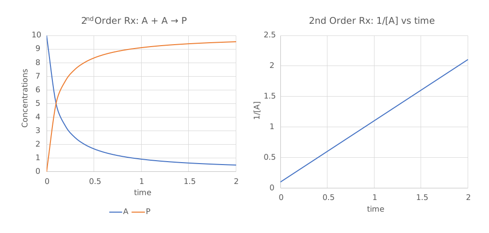
Note that just from a plot of A vs. t, it would be difficult to distinguish a first from a second-order reaction. If the plots were superimposed, you would observe that at the same concentration of A (10, for example), the v_o of a first-order reaction would be proportional to 10, but for a second-order reaction, to 10² or 100. Therefore, the second-order reaction is faster (assuming similarity in the relative magnitude of the rate constants), as indicated by the steeper negative slope of the curve. However, at low A (0.1 example), the v_o of a first-order reaction would be proportional to 0.1, but v_o of a second-order reaction is proportional to 0.1² or 0.01. Therefore, at low A, the second-order reaction is slower.

The interactive graphs below show the first and second-order conversion of reactant A to product. Change the sliders to see how the curves are different.

By comparing these curves, you should see how difficult it is to differentiate between a 1^st and 2^nd order process unless the reaction progresses to almost completion.

Multi-Step Reactions

Reversible First Order Reactions

\begin{equation}
\mathrm{A} \underset{\mathrm{k}_2}{\stackrel{\mathrm{k}_1}{\rightleftarrows}} \mathrm{P}
\end{equation}

Here is the differential equation for dA/dt..

\begin{equation}
\mathrm{v}=\frac{\mathrm{dA}}{\mathrm{dt}}=-\mathrm{k}_1 \mathrm{~A}+\mathrm{k}_2 \mathrm{P}
\end{equation}

Here are the solutions for both A and P as a function of time

\begin{equation}
\begin{gathered}
\mathrm{A}=\frac{\mathrm{A}_0\left(\mathrm{k}_2+\mathrm{k}_1\left[\mathrm{e}^{-\left(\mathrm{k}_1+\mathrm{k}_2\right) \mathrm{t}}\right]\right.}{\mathrm{k}_1+\mathrm{k}_2} \\
\mathrm{P}=\mathrm{A}_0-\left(\frac{\mathrm{A}_0\left(\mathrm{k}_2+\mathrm{k}_1\left[\mathrm{e}^{-\left(\mathrm{k}_1+\mathrm{k}_2\right) \mathrm{t}}\right]\right.}{\mathrm{k}_1+\mathrm{k}_2}\right)
\end{gathered}
\end{equation}

Figure \(\PageIndex{3}\) shows graphs of A and P vs t for this reaction at two different sets of values of k₁ and k₂.

Figure \(\PageIndex{3}\): Graphs of A and P vs t for the reversible reaction A↔P at two different sets of values of k₁ and k₂

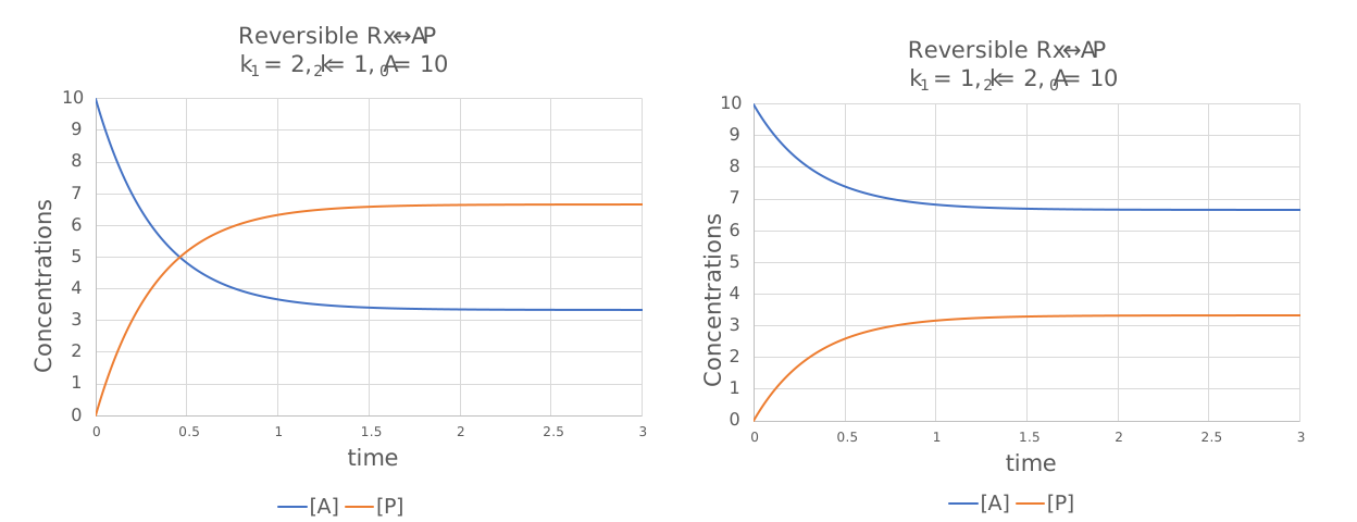
Change the sliders on the interactive graph below of a reversible reaction to see how changing the relative values of the forward and reverse rate constants affects the concentrations at which the concentration plateaus are reached.

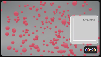
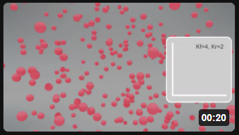
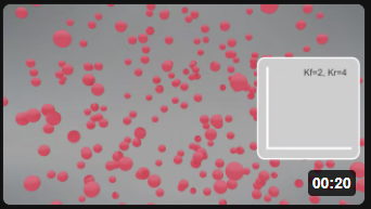
We all grew up on mathematical graphs that give you valuable insight into textual descriptions and data tables from which the graphs were made. These graphs are enhanced when you can use sliders to change constants, as for the reversible reaction A ↔ P above. Even then, you might not infer that when the reaction has reached equilibrium, product is still being made from reactant, and reactant from product, since the equilibrium is dynamic. To add insight into simple and complex reactions, animations showing the continual disappearance of reactants and products are valuable.

This book will incorporate many animations to show the changes in the reactant and product concentrations visually. Hui Liu and Shraddha Nayak (Animation Lab, University of Utah) made all the animations in this book using mathematical solutions to the progress curves for the reactions. Multiple modes of presentation are useful as learners with different backgrounds and preferred ways of learning attempt to understand complex materials.

It is relatively simple to write the differential equations (differential) to show how the rate of disappearance of a reactant A (for example), dA/dt, depends on the concentration of its immediate participants in the reaction. It is not so easy to solve the equations (as we did above) for the progress curve, which shows how [A] changes with time t (i.e., [A] = f(t)). Luckily, many programs have been developed that produce numerical solutions to the differential equations and give progress curve graphs like [A] = f(t). Two interrelated, freely available programs, Copasi and Virtual Cell (Vcell), can solve all the equations for hundreds of cellular reactions simultaneously. They use a format called Systems Biology Markup Language (SBML) for describing and storing computational models. We will use Vcell models in this book as they are straightforward to create. All the coding to describe the reactions is built into Vcell and this book, and hidden from you. All you will see are the output results. You can change the progress curves by moving sliders to change constants and see the resulting changes in graphical outputs.

The VCell models use a reaction diagram that shows all of the interconnected species. The first Vcell model we will run is for the reversible conversion of A to P (A ↔P), which we just discussed and displayed in the graph above. Here is the Vcell reaction diagram and a description of its components.

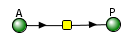
• The reactant A and product P are called species and are shown as green spheres.
• The yellow square indicates a reaction node connecting A to P.
• Lines connect the species that participate in the reaction. The arrows appear unidirectional, BUT the equations describing the concentrations of A and P are derived assuming a reversible reaction with rate constants k_f (forward reaction) and k_r (reverse reaction).

The program calculates A and P as a function of time (i.e., it solves the differential equations for both species). The graphs of concentration vs time are called progress curves. It can also calculate fluxes (J) (velocities) for each species. The flux at any given time is the slope of the concentration vs time curve at any given time. When we get to metabolism, we will talk about fluxes of metabolites through pathways. Also, fluxes are used to describe the rate of movement of solute through membranes. Here is the result of the simulation run in Vcell, exported as an SBML file, and displayed in the book using a program called MiniSideWinder.

---

MODEL

Reversible reaction A ↔ P

Vcell reaction diagram (1-way arrows defined as reversible in actual mathematical model) and chemical equation

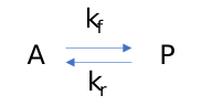
Initial parameter values: k_f = 2,  k_r = 4

Select Load [model name] below

 Select Start to begin the simulation.

Interactive Element

Select Plot to change Y axis min/max, then Reset and Play  |  Select Slider to change which constants are displayed |  Select About  for software information.

Move the sliders to change the constants and see changes in the displayed graph in real-time.

Time course model made using Virtual Cell (Vcell), The Center for Cell Analysis & Modeling, at UConn Health.  Funded by NIH/NIGMS (R24 GM137787); Web simulation software (miniSidewinder) from Bartholomew Jardine and Herbert M. Sauro, University of Washington.  Funded by NIH/NIGMS (RO1-GM123032-04)

---

Animations

The video animations show particles representing A (red) and P (cyan) interconverting in a reversible process with embedded progress curves showing A (red) and P (cyan) vs. time.

Reversible Rx A (red) ↔ B (cyan): kF = kR = 3	Reversible Rx A (red) ↔ B (cyan): kF=4, kR=2	Reversible Rx A (red) ↔ B (cyan): kF=2, kR=4

Consecutive Irreversible First-Order Reactions

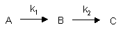
The following differential equations can be written for these reactions:

\begin{equation}
\begin{gathered}
\frac{\mathrm{d} \mathrm{A}}{\mathrm{dt}}=-\mathrm{k}_1 \mathrm{~A} \\
\frac{\mathrm{dB}}{\mathrm{dt}}=\mathrm{k}_1 \mathrm{~A}-\mathrm{k}_2 \mathrm{~B} \\
\frac{\mathrm{dC}}{\mathrm{dt}}=\mathrm{k}_2 \mathrm{~B}
\end{gathered}
\end{equation}

Here are the solutions to the differential equations:

\begin{array}{c}{\mathrm{A}=\mathrm{A}_{0} \mathrm{e}^{-\mathrm{k}_{1} \mathrm{t}}} \\ {\mathrm{B}=\frac{\mathrm{k}_{1} \mathrm{A}_{0}}{\mathrm{k}_{2}-\mathrm{k}_{1}}\left(\mathrm{e}^{-\mathrm{k}_{1} \mathrm{t}}-\mathrm{e}^{-\mathrm{k}_{2} \mathrm{t}}\right)} \\ {\mathrm{C}=\mathrm{A}_{0}-\mathrm{A}-\mathrm{B}=\mathrm{A}_{0}\left[1+\frac{1}{\mathrm{k}_{1}-\mathrm{k}_{2}}\left(\mathrm{k}_{2} \mathrm{e}^{-\mathrm{k}_{1} \mathrm{t}}-\mathrm{k}_{1} \mathrm{e}^{-\mathrm{k}_{2} \mathrm{t}}\right]\right.}\end{array}

Figure \(\PageIndex{4}\) shows graphs of A, B, and C vs. t for these reactions for a fixed value of k₁ and k₂.

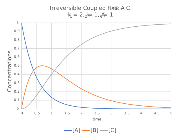
Figure \(\PageIndex{4}\): Graphs of A, B, and C vs. t for the irreversible reactions A → B → C for a fixed value of k₁ and k₂.

Change the sliders on the interactive graph below to see how changing the forward and reverse rate constants affects the curves.

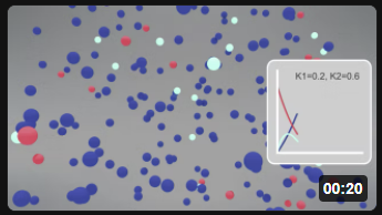
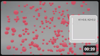
Here are two different animations for the irreversible reaction using different rate constants.

Irreversible Rx A (red) → B (cyan) → C (blue) k1 = 0.2, k2 = 0.6	Irreversible Rx A (red) → B (cyan)→ C (blue) k1= 0.6, k2 = 0.2

Consecutive Reversible First-Order Reactions

You can imagine that solving the equations for the completely reversible reactions of A ↔ B ↔ C would be very difficult. However, writing the differential equations for each step is straightforward and can be done easily in Vcell by choosing the built-in equations for each separate reaction based on mass action. The program can then solve the equations numerically to produce progress curve graphs.

Now let's look at the simulation for the fully reversible reactions A ↔ B ↔ C. Again, the model was built and solved in VCell, and then exported in the system's biology markup language (SBML) format. The interactive graphs are made using a program called miniSideWinder.

A note: Arrows in VCell Diagrams - In the reaction diagram for the reversible reaction A ↔ B ↔ C below, the arrows go in only one direction, left to right, which simply shows that the species are connected. However, in the Vcell program, the equations for the reversible reaction were used to produce the graphs below. To run the simulation of the irreversible reaction, the rate constants for the reverse reaction would be set to 0.

---

MODEL

Reversible reaction A ↔ B ↔ C.

Vcell reaction diagram (1-way arrows defined as reversible in actual mathematical model)

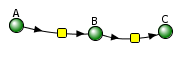
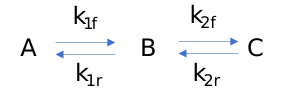
Initial parameter values: k_1f = 0.2, k_1r = 0.1, k_2f = 0.6, k2r = 0.3 A₀ = 1

Select Load [model name] below

 Select Start to begin the simulation.

Interactive Element

Select Plot to change Y axis min/max, then Reset and Play  |  Select Slider to change which constants are displayed |  Select About  for software information.

Move the sliders to change the constants and see changes in the displayed graph in real-time.

Time course model made using Virtual Cell (Vcell), The Center for Cell Analysis & Modeling, at UConn Health.  Funded by NIH/NIGMS (R24 GM137787); Web simulation software (miniSidewinder) from Bartholomew Jardine and Herbert M. Sauro, University of Washington.  Funded by NIH/NIGMS (RO1-GM123032-04)

---

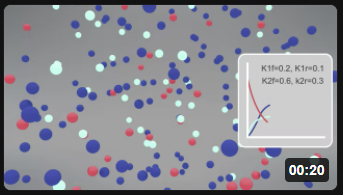
Here is the corresponding animation for the fully reversible reaction A ↔ B ↔ C.

Reversible Rx A (red) ↔ B (cyan) ↔ C Blue) k1f = 0.2, k1r = 0.1; k2f =0.6, k2r = 0.3

 

Summary

(Summary written by Claude, Sonnet 4.6, Anthropic)

This chapter introduces the mathematical and conceptual foundations of chemical kinetics as applied to biochemical reaction systems, beginning with simple single-step reactions and progressing to coupled reversible multi-step schemes that are prerequisites for understanding enzyme-catalyzed reactions.  It begins by establishing the language of calculus for describing reaction rates. Students learn to interpret the derivative (dX/dt) as the instantaneous rate of change in concentration and to use integrals to derive expressions that relate concentration to time. This mathematical framework provides the basis for writing and solving differential equations that describe reaction progress.

Analyzing reaction kinetics requires two complementary experimental approaches. In the initial rate method, the velocity v₀ is measured as the initial slope of a concentration vs. time curve at early time points when [A] ≈ A₀ and has barely changed; v₀ is then plotted as a function of initial reactant concentration. This approach is familiar from enzyme kinetics but sacrifices information about later phases of the reaction. In the integrated rate (progress curve) method, the differential equation d[A]/dt = f([A]) is solved — analytically for simple cases, numerically by computer for complex ones — to yield a function [A] = f(t) that describes the full time course of the reaction. Fitting experimental progress curves to these solutions yields rate constants and mechanistic information about all reaction phases, not just the initial one.

First-order reactions (A → P, rate = k₁[A]) are the simplest and most important class. The differential equation d[A]/dt = −k₁[A] integrates to the exponential decay [A] = A₀e^(−k₁t). Graphically, [A] vs. t is a decaying exponential while ln[A] vs. t is linear with slope −k₁ — the diagnostic test for first-order behavior. Velocity is proportional to [A] at all times: as [A] halves, the rate halves, so the half-life t₁/₂ = 0.693/k₁ is constant and concentration-independent. Second-order reactions (rate = k₂[A]², d[A]/dt = −k₂[A]²) integrate to give 1/[A] = 1/A₀ + k₂t, so a plot of 1/[A] vs. t is linear with slope k₂. At high [A], second-order reactions are faster than first-order ones (velocity ∝ [A]²), but at low [A] they become slower. When one reactant B is present in large excess over A in a bimolecular reaction A + B → P, [B] is effectively constant throughout the reaction, and the apparent rate becomes k₁' = k₂[B] — a pseudo-first-order rate constant — simplifying analysis to the first-order case.

Multi-step reactions require coupled differential equations. For the reversible first-order reaction A ↔ P, d[A]/dt = −k₁[A] + k₋₁[P] and d[P]/dt = k₁[A] − k₋₁[P]. The system approaches equilibrium at a plateau where [P]eq/[A]eq = k₁/k₋₁ = Keq. Importantly, this dynamic equilibrium is not static: forward and reverse fluxes continue at equal rates, so product is continuously being made from reactant and vice versa — a conceptual point easily missed from static graphs but made vivid by particle animations. The ratio k₁/k₋₁ determines the equilibrium position: a larger k₁ relative to k₋₁ drives the reaction further toward product.

Consecutive irreversible reactions A → B → C introduce the concept of a transient intermediate. B first accumulates (because it is being made from A faster than it converts to C) and then depletes (as A is exhausted and B converts to C). The height and timing of the B maximum depend critically on the relative magnitudes of k₁ and k₂: when k₁ >> k₂, B accumulates extensively before slowly draining to C; when k₂ >> k₁, B is consumed almost as fast as it is made and never reaches high concentration. For fully reversible coupled reactions A ↔ B ↔ C, analytical solutions become complex, but differential equations for each species can be written straightforwardly from mass-action kinetics and solved numerically using computational tools. The chapter introduces VCell (Virtual Cell) and COPASI — programs that implement SBML-formatted kinetic models and produce progress curve graphs via numerical integration — as practical tools for visualizing how changing any rate constant (k₁f, k₁r, k₂f, k₂r) shifts the time course and equilibrium concentrations of all species in real time. Interactive sliders and particle animations complement mathematical graphs to build intuition about dynamic equilibria and flux through coupled reaction networks — foundations essential for understanding the more complex kinetic schemes of enzyme catalysis in subsequent chapters.