3.4: Analyses of Protein Structure

Search Fundamentals of Biochemistry

Notes to students and instructors:

This section is placed in Chapter 3 before the in-depth look at protein structure in Chapter 4.  It could be placed in either chapter from a learning and teaching perspective.  Proteins are very complicated.  This section could help students understand the tools used to explore and understand protein structure/function before a deeper dive into structural features found in Chapter 4 and throughout the book.  Alternatively, it could also deepen an acquired understanding of proteins if used at the end of Chapter 4.

This comprehensive section covers topics (such as mass spectrometry, NMR, and molecular dynamics) that might not be broadly discussed or even mentioned in a one-semester survey course. Some of the methods may be more historic and less relevant today.  Instructors can choose parts that are appropriate to their learning goals.

Learning Goals (ChatGPT o1

• Conceptualize Structural Resolution in Protein Analysis:

  • Explain the concept of “resolution” and how different analytical techniques (from low to high resolution) reveal various levels of protein structure and function.

• Master Low-Resolution Analytical Techniques:

  • Describe methods for determining protein concentration (e.g., UV absorbance, dye-binding assays, BCA) and discuss their advantages, limitations, and sources of interference.
  • Outline techniques for amino acid composition analysis, N-/C-terminal analysis, and primary sequence determination, including the use of chemical assays and Edman degradation.

• Understand Spectral Techniques for Structural Insights:

  • Explain how circular dichroism (CD) spectroscopy provides information about secondary structure by differentiating between α-helices, β-sheets, and random coils.
  • Discuss the principles behind fluorescence spectroscopy, including intrinsic versus extrinsic fluorophores, fluorescence quenching, and fluorescence resonance energy transfer (FRET) for studying protein-ligand interactions and conformational changes.
  • Define key fluorescence concepts such as Stokes shift and anisotropy, and how they reflect changes in the protein’s environment or dynamics.

• Grasp Mass Spectrometry for Protein Analysis:

  • Describe the principles of mass spectrometry for protein characterization, including ionization techniques (ESI and MALDI), mass analyzers, and the calculation of molecular weight from m/z values.
  • Differentiate between top-down, bottom-up, and middle-down approaches in proteomic analysis, and explain how peptide mass fingerprinting and tandem MS/MS contribute to protein sequencing and post-translational modification mapping.

• Explore High-Resolution Structural Determination:

  • Compare X-ray crystallography, NMR spectroscopy, and cryo-electron microscopy (cryo-EM) in terms of sample requirements, strengths, limitations, and the type of structural information provided.
  • Discuss how time-resolved crystallography and multidimensional NMR techniques offer insights into protein dynamics and conformational changes.

• Integrate Computational and Dynamic Analyses:

  • Explain the basic principles of molecular mechanics and molecular dynamics (MD) simulations, including the use of force fields to model bonded and nonbonded interactions.
  • Discuss how MD simulations help predict conformational changes, calculate free energy differences (ΔG), and complement experimental data from high-resolution methods.

• Contextualize Proteome Complexity:

  • Define the proteome and discuss the challenges of proteomic analysis due to dynamic protein expression, diverse post-translational modifications, and the wide range of protein abundances.
  • Describe how integrated workflows (e.g., 2D electrophoresis combined with LC-MS/MS) are used in proteomics to identify and quantify proteins in complex biological samples.

• Synthesize Structure/Function Relationships:

  • Connect the information obtained from various analytical techniques to understand how protein structure—from primary sequence to 3D architecture—dictates function.
  • Evaluate how conformational dynamics, ligand binding, and post-translational modifications modulate protein activity and interactions in a cellular context.

These learning goals will enable students to critically assess experimental approaches for studying proteins and to integrate biochemical, biophysical, and computational techniques to elucidate structure/function relationships in biological macromolecules.

Introduction

In the last chapter section, we discussed how to purify a protein (primarily through differential salt precipitation and column chromatography) and how to assess its purity (primarily through various electrophoresis methods) during purification. Now, we want to continue analyzing a "pure" protein to understand its structure and the function conferred by that structure. We need a lot of information to study protein structure/function relationships. Some are "low resolution" characteristics, such as knowing the concentration of a protein. At the highest "resolution" end, we would like to know the 3D structure of a protein with a specific ligand bound to a specific site. Our goal is then to understand proteins at varying levels of complexity or "resolution," some of which are illustrated in Figure \(\PageIndex{1}\).

Figure \(\PageIndex{1}\): Understanding proteins from low to high resolution

Various chemical and spectroscopy analysis techniques are used to achieve the specified level of structural elucidation. Spectral techniques can give us information on concentration (UV absorbance, fluorescence) and secondary structure (CD spectroscopy). Chemical analyses and mass spectroscopy give information on the amino acid composition and/or sequence. More sophisticated techniques (x-ray crystallography, cryoelectron microscopy, NMR spectroscopy) can give us 3D structural information. Each analysis shown in the figure above will be summarized below. 

Sequencing the cDNA can give you some information (amino acid composition, N- and C-terminal amino acids, and the primary structure (omitted from the figure above). Even DNA sequencing won't provide information on post-translational modifications and other covalent processing (e.g., limited proteolysis, disulfide bond formation) that some of the methods below would.

In this section, we will explore some commonly used methods for protein analysis. In previous sections, we learned about the charge and chemical reactivity properties of isolated amino acids in proteins. Analyzing a whole protein is complicated because each amino acid is most often represented multiple times in the sequence. Each protein has an N-terminal and a C-terminal amino acid, as well as secondary structure. Some proteins exist biologically as multisubunit complexes, which adds to the complexity of analyses, since these proteins now have multiple N- and C-terminal ends. In addition, isolated proteins might have chemical modifications (post-translational), which add to the functionalities of the proteins and the complexities of the analyses.

Spectral techniques are widely used to provide information on protein concentration (UV absorbance, fluorescence) and secondary structure (CD spectroscopy). Chemical analyses and mass spectroscopy give information on the amino acid composition and/or sequence. More sophisticated techniques (X-ray crystallography, cryoelectron microscopy, NMR spectroscopy) can give us 3D structural information. More complete descriptions of two techniques, fluorescence spectroscopy and mass spectrometry, are presented, as their use in the analysis of biomacromolecules is underrepresented in curricula. In contrast, their use in actual laboratories becomes increasingly prevalent.

Low-Resolution Analyzes

Protein Concentration

There are multiple methods for determining protein concentrations in samples. Other components of a protein solution may interfere with the assays, so the choice of methods must be carefully determined.

1. Direct mass determination. A known, accurate amount of a dried protein is added to a solution of specific ionic strength and composition. The absorbance at a specific wavelength (usually 280 nm) is measured, and an extinction coefficient at that wavelength (ε1% = absorbance of a 1% protein solution = 1g protein/100 ml solution) is determined. If the protein's molecular weight is known from sequence analysis, a molar absorptivity can be determined. The concentration of the same protein in an unknown pure solution can then be determined. There are several problems with this technique. It requires relatively large amounts of protein to make accurate measurements. An even more difficult problem is that proteins bind water and counter-ions. Even a freeze-dried protein (frozen at -60 ⁰C and placed in a vacuum, which causes sublimation of water and volatile salts in the solution) has probably 10% by weight of bound water (water of hydration).

2. Quantitative amino acid analysis. The protein is hydrolyzed completely to amino acids with 6N HCl. The amino acids are then separated by high-performance liquid chromatography. As amino acids elute from the column, they are reacted with a fluorescent reagent, such as ninhydrin, fluorescamine, or orthophthaldehyde (OPA), to produce a fluorescent amino acid conjugate. The fluorescence intensity of the conjugates is proportional to the concentration of the amino acids in the protein. Before hydrolysis, a known quantity of an amino acid not present in proteins (norleucine, beta-alanine) is added, and its recovery is determined at the end of the hydrolysis and fluorescence conjugation to normalize the recovery of the other amino acids. Several problems are encountered using this technique. Incomplete peptide bond hydrolysis and partial or complete destruction of serine, threonine, tryptophan, and tyrosine occur during the acid hydrolysis. The OH-containing amino acids can be determined by quantifying them at several time points during hydrolysis and extrapolating the concentrations back to zero time. Incomplete reactions with the detecting reagent can also occur.

The most widely used, and perhaps less analytically accurate, are indirect, comparative protein assays based on the chemical properties of amide bonds or the spectrophotometric properties of the side chains Trp, Tyr, and Phe. Unknown concentrations can be determined from a standard curve derived from performing the same reactions or spectrophotometric measurements on a series of solutions of known protein concentration. Below is a discussion of each of these techniques.

3. Modified Lowry protein determination. The Lowry Method is a modification of the biuret method, whose basis is described below. It is, however, much more sensitive. Biuret, as its name implies, derives from combining two urea molecules (bi-ur-et), as shown in the figure (panel A) below.  A violet color results when copper sulfate is added to biuret in a concentrated hydroxide solution. An illustration of the copper (II) complex with biuret is shown in panel B of the figure. This biuret reaction also arises in any compound with three or more peptide bonds. Compare in Figure \(\PageIndex{2}\) the structure of Biuret and a polypeptide (Panel A).

Figure \(\PageIndex{2}\): The biuret reaction for protein quantitation

4. Dye binding assay (Bradford method). This method is based on the binding of the dye Coomassie Brilliant Blue G-250 to proteins, resulting in a change in the dye's absorbance. The structure of the dye is shown in Figure \(\PageIndex{3}\).

Figure \(\PageIndex{3}\): Structures of Coomassie Brilliant Blue R-250 and G-250 (with 2 -CH₃ groups added)

The magnitude of the difference spectra at 595 nm is directly proportional to the protein concentration. The dye in the unbound free state has an absorbance maximum of 465 nm. Bradford initially developed the method (Analytic Biochemistry, 72, 1976), which is available commercially. The dye appears to bind to proteins through hydrophobic and electrostatic interactions with a sulfonic acid group on the dye. The predominant advantage of this method is that it is cheap, simple, rapid, 3x more sensitive than the modified Lowry method, and less susceptible to interference from other compounds. The color fully develops in about 5 minutes, but decreases within 10-15 minutes when the proteins start to precipitate. Precipitation occurs more extensively at higher protein concentrations. Hence, the high-concentration standards will be affected more than the low-concentration standards.

5. Bicinchoninic Acid method (BCA). This method is based on the reduction of Cu⁺⁺ to Cu⁺ by the peptide bond and the chelation of the Cu+ by BCA, which is monitored by absorbance at 562 nm. This method, which has been commercialized, is less prone to interference from other compounds than either the modified Lowry or the dye-binding assay. Two solutions are required: a BCA solution and a copper sulfate solution. The two are mixed to form an apple-green working solution. When protein is added, the resulting Cu⁺ chelates with two molecules of BCA, as shown in Figure \(\PageIndex{4}\).

Figure \(\PageIndex{4}\): BCA analysis for protein quantitation

This results in a purple color, which can be monitored spectrophotometrically at 562 nm. An absorbance at 562 nm of 0.012 per microgram of protein added to the working reagent gives this technique high sensitivity.

6. Absorbance A₂₈₀ or ratios at different wavelengths. This method is based on the fact that the three aromatic acids (Tyr, Phe, Trp) have significant absorbances in the UV. The absorption spectra of the three amino acids as a function of wavelength are shown in Figure \(\PageIndex{5}\). Note the log scale on the y-axis.

Figure \(\PageIndex{5}\): Log absorbance spectra of tyrosine, phenylalanine, and tryptophan

The elution of proteins from chromatography columns is typically monitored by measuring the absorbance of the eluate at 280 nm as it leaves the column, a proxy for protein concentration.  An average protein at a concentration of 1 mg/ml has an A₂₈₀ of about 1. However, only two amino acids absorb significantly at this wavelength. Since proteins have variable numbers of these amino acids, this measurement can only estimate the concentration of an unknown protein.

The Beer-Lambert law shows that the absorbance of a chromophore in solution is given by

\begin{equation}
\mathrm{A}=\epsilon \mathrm{l} \mathrm{c}
\end{equation}

where A is the absorbance at a given wavelength, ε is the molar absorptivity, l is the path length of the cuvette, and c is the concentration (mol/L). Pace et al. have shown that, based on over a hundred measurements on 61 proteins in an aqueous solution, the ε(280), the molar absorptivity at 280 nm, is given by this empirical equation:

\begin{equation}
\epsilon(280)\left(\mathrm{M}^{-1} \mathrm{~cm}^{-1}\right)=(\# \operatorname{Trp})(5,500)+(\# \mathrm{Tyr})(1,490)+(\# \text { cystine })(125)
\end{equation}

Proteins also absorb strongly at wavelengths less than 240 nm. This part of the absorption spectra arises from the above-mentioned amino acids and contributions from His, Met, Cys, and the peptide bond. At these wavelengths, the absorbance is less dependent on the protein's amino acid composition, but it becomes increasingly susceptible to interference from other substances. Contaminating nucleic acids, which absorb maximally at 260 nm, also contribute to the absorbance at 280 nm. Hence, the A₂₈₀/A₂₆₀ ratio can be determined, and the contribution of nucleic acids can be removed through appropriate calculations. Optimal reliability is achieved by measuring A_280/A₂₀₅ values since, at 205 nm, a large fraction of the absorbance due to the peptide bond. pH changes have little effect on the absorbance of the peptide bond but have a much larger effect on Tyr. At high pH, the side-chain hydroxyl is deprotonated (pKa = 10.5), with concomitant changes in A₂₉₅. These changes can be used to follow the titration of the Tyr residues in a protein.

Molecular Weight

Hydrodynamic techniques can estimate molecular weights, including size exclusion chromatography (under denaturing conditions using standards of known molecular weight), ultracentrifugation, and dynamic light scattering. In addition, they can be determined by polyacrylamide gel electrophoresis, again under denaturing conditions using standards. More precisely, it could be determined through protein or cDNA sequence analyses. As described below, mass spectrometry is the most accurate method for smaller proteins.

Specific Amino Acids

Aromatic amino acids can be detected by their characteristic absorbance profiles. As shown in Chapter 3.1: Amino Acids and Peptides, amino acids with specific functional groups can be determined by chemical reactions with specific modifying groups.

Amino Acid Composition

At low resolution, we can determine the amino acid composition of the protein by hydrolyzing it in 6 N HCl at 100 °C under vacuum for various time intervals. After removing the HCl, the hydrolysate is applied to an ion-exchange or hydrophobic-interaction column, and the amino acids are eluted and quantified using known standards. A non-naturally occurring amino acid, like norleucine, is added in known amounts as an internal standard to monitor quantitative recovery during the reactions. The separated amino acids are often derivatized with ninhydrin or phenylisothiocyanate to facilitate their detection. The reaction is carried out for 24, 36, and 48 hours since amino acids with OH (like ser) are destroyed. A time course allows the concentration of Ser at time t=0 to be extrapolated. Trp is also destroyed during the process. In addition, the amide links in the side chains of Gln and Asn are hydrolyzed to form Glu and Asp, respectively.

N- and C-Terminal Amino Acid Analysis

The amino acid composition does not determine the protein's sequence. The N-terminus of the protein can be determined by reacting the protein with fluorodinitrobenzene (FDNB) or dansyl chloride, which reacts with any free amine in the protein, including the epsilon amino group of lysine. The amino group of the protein is linked to the aromatic ring of the dinitrobenzene through an amine and to the dansyl group by a sulfonamide and is hence stable to hydrolysis. The protein is hydrolyzed in 6 N HCl, and the amino acids are separated by TLC or HPLC. Two spots should result if the protein were a single chain with some Lys residues. The labeled amino acid other than Lys is the N-terminal amino acid. The C-terminal amino acid can be determined by adding carboxypeptidases, which cleave amino acids from the C-terminal. A time course must be performed to determine which amino acid is released first. N-terminal analysis can also be done as part of sequencing the entire protein using Edman degradation.

Primary Sequence

Protein Sequencing using Edman Degradation

Edman degradation, developed by Pehr Edman, is a method of sequencing amino acids in a peptide. In this method, the amino-terminal residue is labeled and cleaved from the peptide without disrupting the peptide bonds between other amino acid residues. The reaction is shown in Figure \(\PageIndex{6}\).

Figure \(\PageIndex{6}\): Mechanism of the Edman Degradation

Phenyl isothiocyanate is reacted with an uncharged N-terminal amino group under mildly alkaline conditions to form a cyclical phenylthiocarbamoyl derivative. Under acidic conditions, this terminal amino acid derivative is cleaved to a thiazolinone. The thiazolinone amino acid is then selectively extracted into an organic solvent and treated with acid to form the more stable phenylthiohydantoin (PTH)- amino acid derivative that can be identified by using chromatography or electrophoresis. This procedure can then be repeated to identify the next amino acid.

A major drawback of Edman degradation is that the peptides sequenced in this manner cannot exceed 50-60 residues (and, in practice, are typically under 30). The peptide length is limited because cyclical derivatization does not always go to completion. The derivatization problem can be resolved by cleaving large peptides into smaller peptides before proceeding with the reaction. It can accurately sequence up to 30 amino acids, and modern instruments can achieve over 99% efficiency per amino acid. An advantage of the Edman degradation is that it requires only 10-100 picomoles of peptide for sequencing. The Edman degradation reaction was automated in 1967 by Edman and Beggs to speed up the process, and 100 automated devices were in use worldwide by 1973.

Because the Edman degradation proceeds from the N-terminus of the protein, it will not work if the N-terminus has been chemically modified (e.g., by acetylation or formation of pyroglutamic acid). Sequencing will stop if a non-α-amino acid is encountered (e.g., isoaspartic acid), since the favored five-membered ring intermediate cannot be formed. Edman degradation is generally not useful in determining the positions of disulfide bridges. It also requires peptide amounts of 1 picomole or above for discernible results.

Secondary Structure

The percent and type of secondary structure can be determined using circular dichroism (CD) spectroscopy. In this method, right- and left-circularly polarized light illuminates a protein, which is chiral because it is composed entirely of L-amino acids. (The mirror image would be a protein of the same sequence made of D-amino acids.) Differential absorption of the right and left forms gives a CD spectrum

Circularly polarized light can be made when plane-polarized light of the same amplitude and wavelength meets out of phase by 90⁰. (If they were out of phase by 180⁰, they would cancel.)

• To see an animation of how circularly polarized light can be created, go to this page and select: 1. Superposition of plane-polarized waves 2.

If R and L circularly polarized light of the same wavelength and amplitude are passed through an optically inactive medium, the two waves combine (vectorially) to produce plane-polarized light.

• To see an animation of how circularly polarized light can be created, go to this page and select 1. Superposition of circularly polarized waves

Optical activity is observed only when the environment in which a transition occurs is asymmetric.

The peptide (amide) bond absorbs UV light in the range of 180 to 230 nm (far-UV range), so this region of the spectra gives information about the protein backbone and, more specifically, the secondary structure of the protein. The main electronic energy transitions are n → π* at 220 nm and π → π * at 190 nm for the peptide bond. There is a contribution from aromatic amino acid side chains, but it is small, given the large number of peptide bonds. The lone pair on the nitrogen adjacent to the pi bond can be considered rehybridized from sp³ to sp², allowing for conjugation of the p electrons (which lowers the energy of the electrons). The Hückel diagram shown in Figure \(\PageIndex{7}\) below shows three molecular (not atomic) orbitals generated from the three atomic p orbitals.

Figure \(\PageIndex{7}\): Hückel molecular orbitals for the peptide bond

The middle one (with one node) has energy similar to the separate atomic p orbitals and is considered a nonbonding molecular orbital. This is consistent with the lone nonbonding pair on the nitrogen atom.

The peptide bonds in a protein's asymmetric environment will absorb light in this wavelength range (promoting electrons to higher energy levels). In different secondary structures, the peptide bond electrons absorb right- and left-circularly polarized light differently (for example, they exhibit different molar absorptivities). Hence, α, β, and random coil structures exhibit distinguishable far-UV CD spectra.

To see an animation of circularly polarized light, go to this page and select 1. Circularly Polarized Waves

Stated in another way, if plane-polarized light, which is a superposition of right and left circularly polarized light, passes through an asymmetric sample, which absorbs right and left circularly polarized light differently (i.e, they display circular dichroism), then the light passing through the sample after vector addition of the right and left circularly polarized light gives elliptically polarized light.

To see an animation of elliptically polarized light, go to this page and select 2. Plane-polarized waves in a medium with circular dichroism

If the chiral molecules also have a different index of refraction for R and L circularly polarized light, an added effect is the rotation of the angle of the elliptically polarized light. The far-UV CD spectrum of the protein is sensitive to its main chain conformation. The CD spectra of alpha and beta secondary structures are shown in Figure \(\PageIndex{8}\).

Figure \(\PageIndex{8}\): CD spectra of alpha, beta, and random coil structures in proteins

Protein side chains also find themselves in such an asymmetric environment. If irradiated with circularly polarized UV light in the range of 250-300 nm (near UV), differential absorption of right and left circularly polarized light by the aromatic amino acids (Tyr, Phe, Trp) and disulfide bonds occurs, and a near UV CD spectra result. Suppose a protein's near-UV CD spectra are taken under two different sets of conditions, and the spectra differ. In that case, it can be inferred that the environment of the side chains differs, and hence the proteins have somewhat different conformations. It will not provide information about the backbone's secondary structure, as it requires lower wavelengths for absorption. Instead, it can show differences in tertiary structure.

Analysis of Proteins Using Fluorescence Spectroscopy

Fluorescence spectroscopy is widely used to study many aspects of protein chemistry. Although this technique is not often used in lower-level undergraduate classes, it has become so important in the study of biomolecules that a detailed explanation is necessary.

When molecules absorb energy, electrons are promoted to higher electronic energy states. This is the basis of absorption spectroscopy. These excited-state electrons can return to the ground state in processes that don't emit photons of light (ie, nonradiative processes) or radiative processes that emit light. In simple absorption spectroscopy, excited-state electrons relax to the ground state through collisions. In radiative deexcitation, light is emitted. This process of light emission is called luminescence, which can be divided into two categories:

• fluorescence: If one electron from a ground state electron pair is excited to a higher energy state, the excited electrons can still be spin paired with their ground state counterpart - i.e., they have opposite spins. The excited electron can return to the ground state without reversing its spin. (The excited state is a singlet state with S, the total spin state, given the formula S = 2s +1, where s = 0 (sum of +1/2 and -1/2) and S = 1 for a singlet.) This process, which results in rapid photon emission, is "spin allowed." The photon emission rate is about 108 s^-1, resulting in a lifetime (the average time between excitation and emission) of the excited state of about 10 ns.
• phosphorescence: If, in contrast to the above case, the spin of the excited electron is flipped, then its transition back to the ground state is "spin forbidden" since the excited state electron and its ground state counterpart have the same spin state. (The excited state is a triplet state with S, the total spin state, given by the formula S = 2s +1, where s = 1 (1/2 + 1/2) and S = 3 for a triplet. Hence, this transition occurs slowly (in the ms-s range). Toys that glow in the dark display even longer phosphorescence lifetimes. (Note: This guide will concentrate on fluorescence.)

Competing with the two deexcitation processes are nonradiative processes (such as through collisions). Given these competing processes, it might be expected that phosphorescence in liquid solutions at room temperature might not be detectable.

Molecules that fluoresce are typically aromatic, which absorb readily in the UV and visible light regions. Common fluorophores are quinine, found in tonic water (observe the faint blue glow at the surface when placed in direct sunlight), and fluorescein and rhodamine, two fluorophores often added to antifreeze. Atoms are usually nonfluorescent, except europium and terbium ions from the lanthanide series. These fluoresce when electronic transitions occur between f orbitals, which are shielded from solvent relaxation by the filled 5s and 5p orbitals.

Among biological molecules, some, especially macromolecules with aromatic groups, fluoresce. These groups are called intrinsic fluorophores and, in proteins, include the side chains of the aromatic amino acids tryptophan, tyrosine, and phenylalanine. The indole side chain of tryptophan is the most fluorescent, and its emission spectrum, which is sensitive to solvent conditions, is often blue-shifted when the ring is buried and red-shifted when solvent-exposed. Nucleic acids, although they also contain aromatic bases, are poor fluorophores. Many biological molecules can be made fluorescent by covalently modifying them (via nucleophilic groups on the biological molecule) with exogenously added fluorophores, such as fluorescein isothiocyanate, rhodamine isothiocyanate, or dansyl chloride. These are called extrinsic fluorophores. These include molecules that bind noncovalently to structures such as ds-DNA (ethidium bromide) or lipid membranes (diphenylhexatriene). Some biological fluorophores are substrates for enzyme reactions. Examples include oxidized flavins (FAD, FMN) and the reduced form of NAD (i.e., NADH). Another type of useful fluorophore is an indicator, whose fluorescent properties change with a parameter such as pH or [Ca2+].

The electronic transitions that occur during fluorescence can be represented by a Jablonski diagram as shown in the two-part Figure \(\PageIndex{9}\) (A and B) below.

Figure \(\PageIndex{9}\): Jablonski diagram and associated excitation and emission spectra. After Van Holde, et al. Principles of Physical Biochemistry, Pearson Prentice Hall (2006)

In panel A, the ground and first excited electronic states are shown. Each electronic state has multiple vibrational energy levels 0, 1, 2, ... and 0', 1', 2', ... This simple diagram ignores quenching of fluorescence, resonance energy transfer, etc. The transitions, represented by vertical lines, are considered to be instantaneous. They take about 10^-15 s, so the nuclei don't move during that time. The ground-state electron is considered in the zero vibrational level, so thermal energy is insufficient to promote it to the next vibrational level. When light is absorbed, the electron is promoted to a higher vibrational level within a higher electronic level. Usually, the excited electrons relax quickly (< 1 ps) to the lowest vibrational level of S1 or S2 through internal conversion. Fluorescence emission may occur from the lowest vibrational state of S1 to any of the vibrational states of So. Hence, the photon emitted is lower in energy (longer in wavelength) than the absorbed photon. Also, since both processes involve the movement of an electron to different vibrational levels, with absorption or emission of a photon, and nonradiative vibrational relaxation within those levels, the emission spectra are often the mirror image of the absorption spectra. (This assumes that the vibrational levels in So and S1 are similarly spaced. Alternatively, electrons in S1 may flip their spin and convert to the T1 state via intersystem crossing, leading to phosphorescence.

Panel B above shows blue lines for individual absorbances and red lines for emissions. Note that the excitation from 0 to 8' has the highest energy of absorption (lowest wavelength) but gives little intensity as it would occur with low frequency. If you were to draw a line over the tops of the lines in panel B, you would get simple excitation and emission spectra, which would be mirror images of each other. The emission peak is at a longer wavelength since energy was lost on vibrational, nonradiative relaxation of the excited electron. The difference in peak excitation and emission wavelengths is called the Stokes Shift. This shift is greatest for fluorophores in polar environments. Inferences can be made considering the disposition of a side chain (buried or surface) if changes in fluorescence properties (intensity, Stokes' shift) are noted on protein denaturation. Also, many probes are weakly fluorescent in aqueous solution but fluoresce intensely in nonpolar media (e.g., bound to a hydrophobic pocket in a protein, bilayer, or lipoprotein).

Emission spectra are usually independent of excitation wavelength (Kasha's rule). This occurs because the excited state rapidly relaxes into the lowest vibrational energy level. There are also exceptions to the mirror image rule. Deviations arise from a change in the geometry of nuclei in the excited state of the molecule. This may occur if the lifetime of the S1 state is long, allowing time for motion before emission.

An example is p-terphenyl in cyclohexane, where the rings become more coplanar in the excited state. Since there is an electron shift in the excited state, a complex between the excited fluorophore and another solution component may arise (charge-transfer complex). Alternatively, some fluorophores form dimers (e.g., pyrene) at higher concentrations. At high concentrations, changes in the emission spectra occur, arising from excited-state dimers or excimers. Acridine shows two emission spectra at different pHs, arising from changes in the pKa on excitation (5.45 to 10.7). Finally, exciting a fluorophore at different wavelengths (EX 1, EX 2, EX 3) does not change the emission profile. Still, it does produce variations in fluorescence emission intensity (EM 1, EM 2, EM 3) that correspond to the amplitude of the excitation spectrum.

Fluorophores can chemically modify nucleophilic side chains such as lysines and cysteines. Changes in intrinsic fluorescence in proteins can be used to measure ligand binding, conformational changes in the protein during binding interactions, changes in solution conditions, and protein denaturation. Let's explore a few fluorescence methods widely used to explore protein structure and function.

Fluorescence Quenching

Some chemical species (for example, iodide and monomeric, unpolymerized acrylamide), when added to a protein solution, can decrease the fluorescence of an intrinsic, surface-accessible fluorophore, such as the tryptophan side chain, providing information on the local environment of the intrinsic fluorophore (for example, tryptophan side-chain accessibility). For example, a buried tryptophan or probe will show little change in fluorescence intensity in the presence of a large, polar quencher. In contrast, a surface tryptophan or probe will show a significant decrease in fluorescent intensity. It is somewhat amazing that O_2, when added to a solution under increasing pressure, can quench the fluorescence of even buried tryptophan side chains, implying minimal diffusional barriers to O₂ access. This suggests significant conformational flexibility of the protein.

Quenching can be dynamic, occurring when the quencher collides with the intrinsic fluorophore, or static, when the quencher binds to a site near the fluorophore as a prelude to quenching.

Collisional quenching is described by the Stern-Volmer equation.

\begin{equation}
\frac{F_{0}}{F}=1+k_{q} \tau_{0}[Q]=1+K_{D}[Q]
\end{equation}

where F_o and F are the fluorescent intensities in the absence and presence of the quencher, k_q is the biomolecular quenching constant, τ_o is the lifetime of the fluorophore in the absence of the quencher, and [Q] is the concentration of the quencher. k_qτ_o = K_D is the Stern-Volmer quenching constant.

A plot of F_o/F vs [Q] is linear, with a slope of K_D. 1/K_D is the quencher concentration at which F_o/F = 2, or 50% of the fluorescence intensity, is quenched. A linear plot indicates a single class of fluorophores, all of which are equally accessible to the quencher. A nonlinear plot would be found for the quenching of tryptophan fluorescence in proteins by charged or polar quenchers for proteins with more than one tryptophan, and in which some are buried. Static quenching also results in a linear SV plot. Different dependencies on temperature and viscosity can distinguish dynamic and static quenching. Since dynamic quenching depends on diffusion, higher temperatures result in higher diffusion coefficients; therefore, k_q should increase with temperature. If static quenching is involved, higher temperatures will probably reduce complex formation.

Fluorescence Resonance Energy Transfer (FRET)

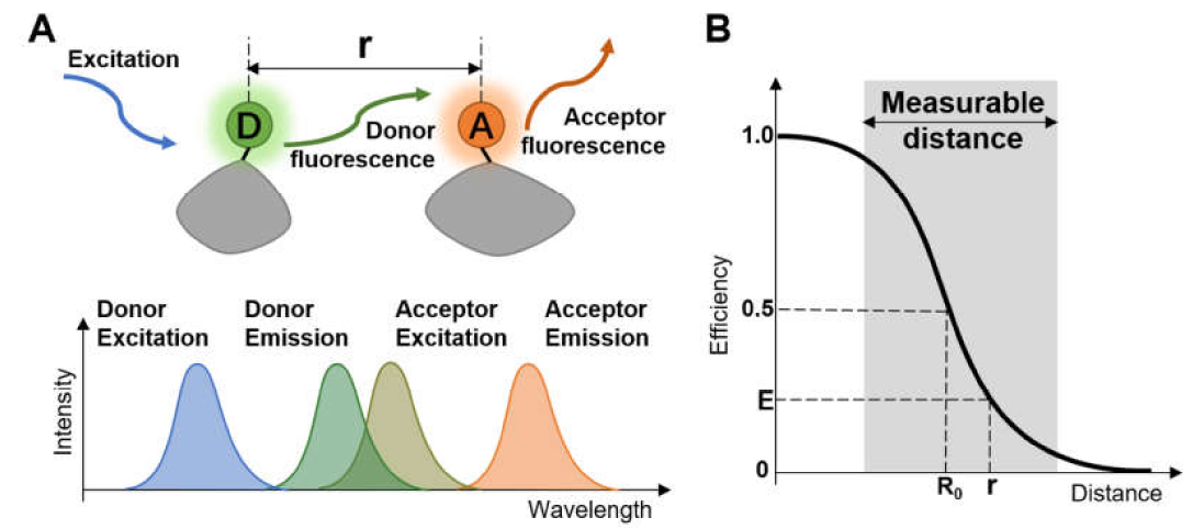
If an absorbing species is near an excited-state fluorophore, and if the emission spectrum of the fluorophore overlaps the absorption spectrum of the second species, coupling of the two dipoles can occur, and energy can be transferred from the excited state of the fluorophore (donor D) to the second absorbing species (acceptor A). This energy transfer occurs through dipole coupling, not through the trivial emission and absorption of a photon. No photon is produced. This process is called fluorescence resonance energy transfer (FRET). Efficiency, E, of FRET for a single donor/acceptor pair at a fixed distance is given by:

\begin{equation}
\mathrm{E}=\frac{\mathrm{R}_{0}^{6}}{\left(\mathrm{R}_{0}^{6}+\mathrm{r}^{6}\right)}=\frac{1}{1+\left(\frac{\mathrm{r}}{\mathrm{R}_{0}}\right)^{6}}
\end{equation}

R_o is the Förster distance (or radius) with a 50% transfer efficiency, and r is the distance between the donor and acceptor. R_o measures the spectral overlap of the donor and acceptor (for which most biological macromolecules have a value of 30-60 angstroms). This equation shows that efficiency depends on 1/r^6, making FRET exquisitely sensitive to distance. Figure \(\PageIndex{10}\) below illustrates FRET and its distance dependency.

Figure \(\PageIndex{10}\): Fluorescence Resonance Energy Transfer (FRET) Qiao, Y.; Luo, Y.; Long, N.; Xing, Y.; Tu, J. Single-Molecular Förster Resonance Energy Transfer Measurement on Structures and Interactions of Biomolecules. Micromachines 2021, 12, 492. https://doi.org/10.3390/mi12050492Creative Commons Attribution (CC BY) license (https://creativecommons.org/licenses/by/4.0/).

Anisotropy or polarization

These measure the extent of rotation of the fluorophore during its fluorescent lifetime. If a small fluorophore binds to a large molecule, its rotational diffusion constant decreases, and its anisotropy increases, as illustrated in Figure \(\PageIndex{11}\).

Figure \(\PageIndex{11}\): Fluorescence anisotropy and rotational diffusion of a fluorophore. -2563-4Creative Commons Attribution 4.0 International License (http://creativecommons.org/licenses/by/4.0/).

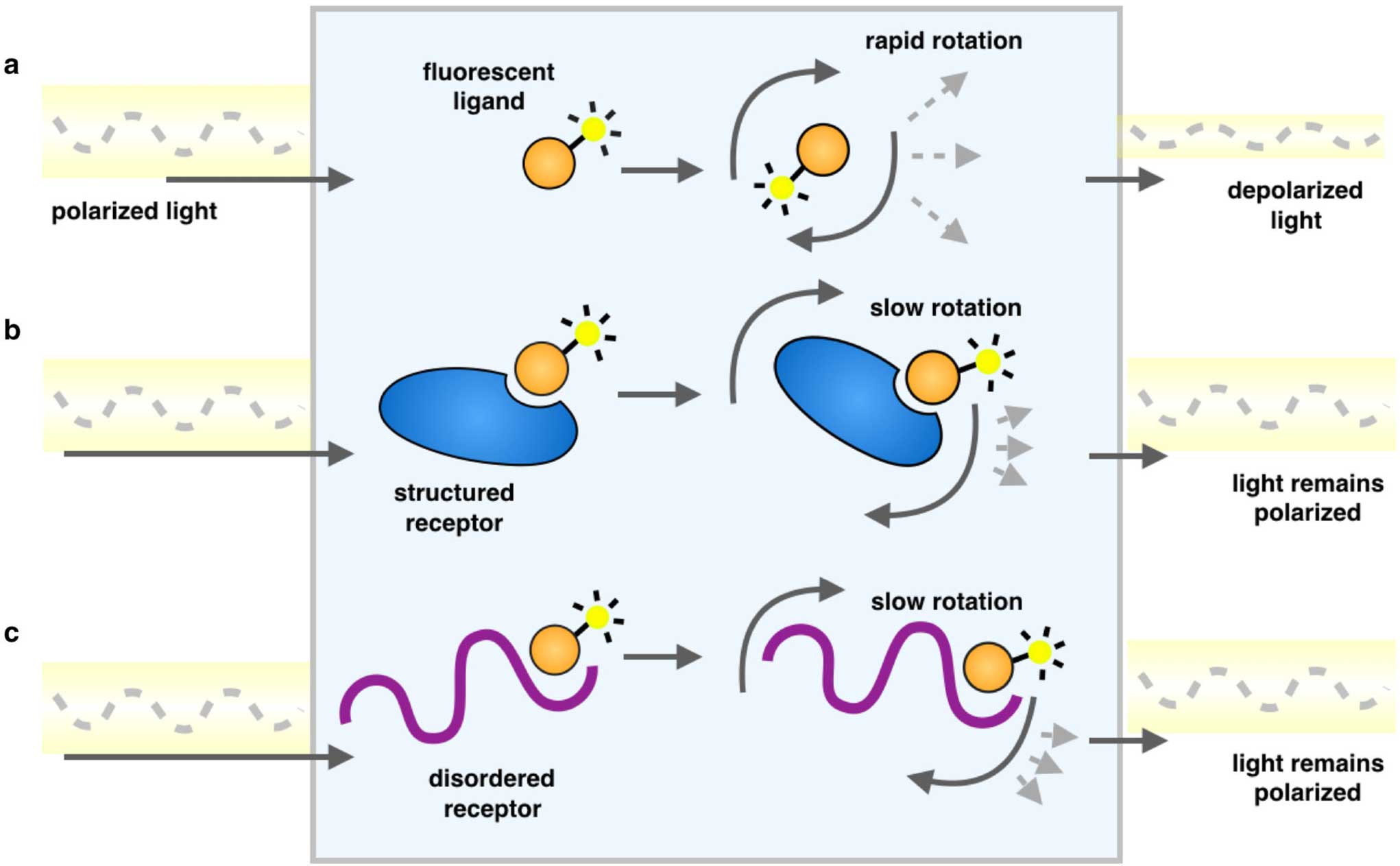
Schematic representation of a fluorescence polarization experiment. As a result of the rapid tumbling of molecules in solution, when a fluorescently labeled ligand is excited with plane-polarized light, the resulting emitted light is largely depolarized (a). Upon binding another species, a larger proportion of the emitted light remains in the same plane as the excitation energy because the rotation is slowed as the effective molecular size increases, whether it is an ordered molecular structure (b) or one that is disordered (c)". Since viscosity decreases rotational diffusion rates, changes in fluorescence (such as inside a bilayer) can be inferred from these measurements. For example, membranes more enriched in saturated fatty acids should show increased anisotropy of a hydrophobic, fluorescent probe compared to the same probe in a bilayer enriched in polyunsaturated fatty acids.

Analysis of Protein Using Mass Spectrometry

Mass spectrometry supplants traditional methods (see above) to determine a protein's molecular mass and structure. Its power comes from its exquisite sensitivity and modern computational methods for determining structure by comparing ion fragment data with databases of known protein structures. In mass spectrometry, a molecule is first ionized in an ion source. An electric field then accelerates the charged particles into a mass analyzer, where they are subjected to an external magnetic field. The external magnetic field interacts with the magnetic field generated by the charged particles' motion, deflecting them. The deflection is proportional to the mass-to-charge ratio, m/z. Ions then enter the detector, which is usually a photomultiplier. Sample introduction into the ion source occurs through simple diffusion of gases and volatile liquids from a reservoir, by injecting a liquid sample containing the analyte via a fine mist, or, for very large proteins, by desorbing a protein from a matrix using a laser. Complex mixtures are analyzed by coupling HPLC to mass spectrometry in an LC-MS system.

There are many methods for ionizing molecules, including atmospheric pressure chemical ionization (APCI), chemical ionization (CI), and electron impact (EI). The most common methods for protein/peptide analyses are electrospray ionization (ESI) and matrix-assisted laser desorption ionization (MALDI).

Electrospray ionization (ESI)

The analyte, dissolved in a volatile solvent such as methanol or acetonitrile, is injected into the ion source through a fine stainless steel capillary at a low flow rate. A high voltage (3-4 kV) is applied to the capillary, giving it a positive charge relative to the oppositely charged electrode. The flowing liquid becomes charged with the same polarity as the polarity of the positively charged capillary. The high field leads to the emergence of the sample as a charged aerosol spray of charged microdrops, thereby reducing electrostatic repulsions within the liquid. This method uses electrical energy to produce the aerosol, rather than mechanical energy to produce a liquid aerosol, as in a perfume atomizer. Surrounding the capillary is a flowing gas (nitrogen) that helps move the aerosol toward the mass analyzer. As the volatile solvent evaporates, the microdrops become smaller, increasing the positive charge density on them. Eventually, electrostatic repulsions cause the drops to explode in a series of steps, ultimately producing the analyte devoid of solvent. This gentle ionization method produces analytes that are not cleaved but ready for introduction into the mass analyzer.

Proteins emerge from this process with a roughly Gaussian distribution of positive charges on basic side chains. You studied mass spectra of small molecules induced by electron bombardment in organic chemistry. This produces ions with a +1 charge as an electron is stripped from the neutral molecule. The highest m/z peak in the spectrum corresponds to the parent ion, M⁺. The highest m/z ratio detectable in the mass spectrum is in the thousands. However, large peptides and proteins with high molecular mass can be detected and resolved because their ions carry a charge greater than +1. In 2002, John Fenn was awarded a Nobel Prize in Chemistry for developing and using ESI to study biological molecules.

Figure \(\PageIndex{12}\) shows an example of an ESI spectrum of apo-myoglobin.

Figure \(\PageIndex{12}\): ESI mass spectrum of apo-myoglobin

Note the roughly Gaussian distribution of the peaks, each representing the intact protein with charges differing by +1. Proteins acquire positive charges by protonating amino acid side chains and by charges induced during electrospray. Based on the amino acid sequence of myoglobin and the assumption that the pKas of the side chains are the same in the protein as for isolated amino acids, the calculated average net charges of apomyoglobin (apoMb) would be approximately +30 at pH 3.5, +20 at pH 4.5, +9 at pH 6, and 0 at pH 7.8 (the calculated pI). The mass spectrum below was obtained by direct injection of apoMb into the MS in 0.1% formic acid (pH 2.8)—charges on the peptide result from those present before the electrospray and those induced during the process.

The protein's molecular mass can be determined by analyzing two adjacent peaks, as shown in Figure \(\PageIndex{13}\).

Figure \(\PageIndex{13}\): m/z ratio for two adjacent peaks in the mass spectrum of a protein

Suppose M is the molecular mass of the analyte protein, and n is the number of positive charges on the protein represented in a given m/z peak. In that case, the following equations give the molecular mass M of the protein for each peak:

\begin{equation}
\begin{gathered}
\mathrm{M}_{\text {peak } 2}=\mathrm{n}(\mathrm{m} / \mathrm{z})_{\text {peak } 2}-\mathrm{n}(1.008) \\
\mathrm{M}_{\text {peak } 1}=(\mathrm{n}+1)(\mathrm{m} / \mathrm{z})_{\text {peak } 1}-(\mathrm{n}+1)(1.008)
\end{gathered}
\end{equation}

where 1.008 is the atomic weight of H. Since there is only one value of M, the two equations can be set equal to each other, giving:

\begin{equation}
\mathrm{n}(\mathrm{m} / \mathrm{z})_{\text {peak } 2}-\mathrm{n}(1.008)=(\mathrm{n}+1)(\mathrm{m} / \mathrm{z})_{\text {peak } 1}-(\mathrm{n}+1)(1.008)
\end{equation}

Solving for n gives:

\begin{equation}
\mathrm{n}=\frac{(\mathrm{m} / \mathrm{z})_{\mathrm{peak} 1}-(1.008)}{(\mathrm{m} / \mathrm{z})_{\mathrm{peak} 2}-(\mathrm{m} / \mathrm{z})_{\mathrm{peak} 1}}
\end{equation}

Knowing n, the molecular mass M of the protein can be calculated for each m/z peak. The best value of M can then be determined by averaging the M values determined from each peak (16,956 from the above figure). For peaks from m/z of 893-1542, the calculated values of n ranged from +18 to +10.

Matrix-assisted laser desorption ionization (MALDI)

This technique for larger biomolecules (proteins and polysaccharides) involves mixing the analyte with an absorbing matrix. Laser excitation of the matrix leads to energy transfer, resulting in ionization and the "launching" of the matrix and analyte in ion form from the solid mixture. Parent ion peaks of (M+H)⁺ and (M-H)^- are formed.

The Mass Analyzer separates the created ions based on m/z ratios. Let's consider two: the quadrupole ion trap and the time-of-flight.  There are several general types of mass analyzers, including magnetic sector, time-of-flight, quadrupole, and ion trap.

Quadrupole ion trap (used in ESI) - A complex mixture of ions can be contained (or trapped) in this mass analyzer. Two common types are linear and 3D quadrupole. If a dipole has two poles (+ and  -) separated by some distance, then a quadrupole has four poles (+, -, +, and -) arranged geometrically such that each + has a - on each side and vice versa. Figure \(\PageIndex{14}\) below shows linear and 3D quadrupoles.

Figure \(\PageIndex{14}\): Linear and 3D quadrupoles

As dipoles display positive and negative charge separation on a linear axis, quadrupoles have either opposite electrical charges or opposite magnetic fields at the opposing ends of a square or cube. In charge separation, the monopole (sum of the charges) and dipoles cancel to zero, but the quadrupole moment does not. The quadrupole traps ions using a combination of fixed and alternating electric fields. The trap contains helium at 1 mTorr. For the 3D trap, the ring electrode has an oscillating RF voltage, which keeps the ions trapped. The end caps also have an AC voltage. Ions oscillate in the trap at a "secular" frequency determined by the RF voltage frequency and, of course, the m/z ratio. By increasing the amplitude of the RF field, the ion motion in the trap becomes destabilized, leading to ion ejection into the detector. When the secular frequency of ion motion matches the applied AC voltage across the end cap electrodes, resonance occurs, increasing the ions' motion amplitude and allowing leakage out of the ion trap into the detector.

Tandem Mass Spectrometry (MS/MS): Quadrupole mass analyzers, which can select ions of varying m/z ratios in the ion traps, are commonly used in tandem mass spectrometry (MS/MS). In this technique, the selected ions are further fragmented into smaller ions by collision-induced dissociation (CID). When performed on all of the initial ions present in the ion trap, the sequence of a peptide/protein can be determined. This technique usually requires two mass analyzers with a collision cell in between, where selected ions are fragmented by collision with an inert gas. Using a quadrupole ion trap, it can also be done in a single mass analyzer.

In time-of-flight (TOF) mass spectrometry (used in MALDI), a long tube determines the time required for ion detection. The small molecular mass ions reach the detector the fastest.

Sequence Determination Using Mass Spectrometry

In a typical MS/MS experiment to determine a protein sequence, a protein is cleaved into protein fragments using an enzyme such as trypsin, which cleaves on the carboxyl side of Lys and Arg residues. The average protein size in the human proteome is approximately 50,000. If the average molecular mass of an amino acid in a protein is around 110 (18 subtracted since water is released on amide bond formation), the average number of amino acids in the protein would be around 454. If 10% of the amino acids are Arg and Lys, then on average, there would be approximately 50 Lys and Arg, and hence 50 tryptic peptides of average molecular mass 1000. The fragments are introduced in the MS, where a peptide fragment fingerprint analysis can be performed. The molecular weights of the fragments can be determined and compared with those of known peptide digestion products from known proteins to identify the analyte protein.

Ions with the original N terminus are denoted as a, b, and c, while ions with the original C terminus are denoted as x, y, and z. c and y ions gain an extra proton from the peptide to form positively charged -NH₃⁺ groups. Figure \(\PageIndex{15}\) below shows peaks for a 4-amino acid peptide fragmentation pattern

Figure \(\PageIndex{15}\): 4-amino acid peptide fragmentation peaks. https://commons.wikimedia.org/wiki/F...gmentation.gif.   Creative Commons Attribution-Share Alike 3.0 Unported

Ions with the original N terminus are denoted as a, b, and c, while ions with the original C terminus are denoted as x, y, and z. c and y ions gain an extra proton from the peptide to form positively charged -NH₃⁺ groups. The ions observed depend on many factors, including the peptide sequence, its original charge, the collision energy used to induce fragmentation, etc. Low energy fragmentation of peptides in ion traps usually produces a, b, and y ions, along with peaks resulting from loss of NH₃ (a*, b*, and y*) or H₂O (ao, bo, and yo). No peaks resulting from the fragmentation of side chains are observed. Fragmentation at two sites in the peptide (usually at the b and y sites in the backbone) forms an internal fragment.

The y1 peak represents the tryptic peptide's C-terminal Lys or Arg (in this example). Peak y2 has one more amino acid than y1, and the molecular mass difference identifies the extra amino acid. Peak y3 is likewise one amino acid larger than y2. All three y fragment peaks have a common Lys/Arg C-terminal, and the charged fragment contains the C-terminal end of the original peptide. All b fragment peaks for a given peptide contain a common N-terminal amino acid, with b1 the smallest. Note that the subscript represents the number of amino acids in the fragment. By identifying b and y peaks, the actual sequence of small peptides can be determined. Usually, spectra are matched to databases to identify the structure of each peptide and, ultimately, that of the protein. The actual m values for fragments can be calculated as follows, where (N is the molecular mass of the neutral N terminal group, (C) is the molecular mass of the neutral c terminal group, and (M) is the molecule mass of the neutral amino acids. (For N-terminal amino acid, add 1 H. For C terminus, add OH.)

• a: (N)+(M)-CHO
• b: (N)+(M)
• y: (C)+(M)+H (note in the figure above that the amino terminus of the y peptides has an extra proton in the +1 charged peptides.)

m/z values can be calculated from the m values by adding the mass of the extra proton to the overall z, if the overall charge is +1, etc.

For example, from these MW values, the human Glu1- fibrinopeptide B sequence can be determined from MS/MS spectra shown in an annotated form in Figure \(\PageIndex{16}\). Note that most of the b peaks are b*, resulting from the loss of NH₃ from the N terminus.

Figure \(\PageIndex{16}\): Annotated MS/MS spectra of human Glu1- fibrinopeptide B

Now, let's step back and get a broader picture of structure analysis by mass spectrometry. In general, proteins are analyzed either in a "top-down" approach, in which they are analyzed intact, or in a "bottom-up" approach, in which they are first digested into fragments. An intermediate "middle-down" approach, in which larger peptide fragments are analyzed, may also be used. However, the top-down approach is mostly limited to low-throughput single-protein studies due to issues in handling whole proteins, their heterogeneity, and the complexity of their analyses.

In the second approach, referred to as the "bottom-up" MS, proteins are enzymatically digested into smaller peptides using a protease such as trypsin, which cleaves peptide chains mainly at the carboxyl side of lysine or arginine, except when either is followed by proline. It is used for numerous biotechnological processes. The process is commonly referred to as trypsin proteolysis or trypsinization, and proteins that have been digested/treated with trypsin are said to have been trypsinized.

Subsequently, these peptides are introduced into the mass spectrometer and identified by peptide mass fingerprinting or tandem mass spectrometry. Hence, this approach uses peptide-level identification to infer the presence of proteins pieced back together via de novo repeat detection. The smaller and more uniform fragments are easier to analyze than intact proteins and can be also determined with high accuracy, this "bottom-up" approach is therefore the preferred method of studies in proteomic studies. A further approach that is beginning to be useful is the intermediate "middle-down" approach, in which proteolytic peptides larger than the typical tryptic peptides are analyzed.

Proteins of interest are usually part of a complex mixture of multiple proteins and molecules, which coexist in the biological medium. This presents two significant problems. First, the two ionization techniques used for large molecules are effective only when the mixture contains roughly equal amounts of the constituents. At the same time, different proteins tend to be present in widely differing amounts in biological samples. If such a mixture is ionized using electrospray or MALDI, the more abundant species tend to "drown" or suppress signals from less abundant ones. Second, the mass spectrum from a complex mixture is very difficult to interpret due to the overwhelming number of mixture components. This is exacerbated by the fact that a protein's enzymatic digestion yields multiple peptide products.

In light of these problems, methods such as one- and two-dimensional gel electrophoresis and high-performance liquid chromatography are widely used to separate proteins. The first method fractionates whole proteins via two-dimensional gel electrophoresis (Figure 3.31). The first dimension of 2D gel electrophoresis is isoelectric focusing (IEF). In this dimension, the protein is separated by its isoelectric point (pI), and the second dimension is SDS-polyacrylamide gel electrophoresis (SDS-PAGE). This dimension separates proteins based on their molecular weight. Once this step is complete, in-gel digestion proceeds.

In some situations, combining both of these techniques may be necessary. Gel spots identified on a 2D Gel are usually attributable to one protein. If protein identity is desired, the in-gel digestion method is usually used, in which the protein spot of interest is excised and proteolytically digested. The peptide masses resulting from the digestion can be determined by mass spectrometry using peptide mass fingerprinting. If this information does not allow unequivocal protein identification, its peptides can be subject to tandem mass spectrometry for de novo sequencing. Small changes in mass and charge can be detected with 2D-PAGE. The disadvantages of this technique are its small dynamic range compared to other methods. Some proteins are still difficult to separate due to their acidity, basicity, hydrophobicity, and size (too large or too small).

The second method, high-performance liquid chromatography (HPLC/MS), is used to fractionate peptides after enzymatic digestion. Characterization of protein mixtures using HPLC/MS is also called shotgun proteomics and MuDPIT (Multi-Dimensional Protein Identification Technology). One or two steps of liquid chromatography fractionate a peptide mixture that results from the digestion of a protein mixture. The chromatographic eluant can be directly introduced into the mass spectrometer via electrospray ionization or deposited onto a series of small spots for later MALDI mass analysis.

Figure \(\PageIndex{17}\) shows the general schema for analyzing proteins by mass spectrometry.

Figure \(\PageIndex{17}\): Schematic of Protein Fingerprinting by Mass Spectrometry. Philippe Hupé - Emmanuel Barillot, Laurence Calzone, Philippe Hupé, Jean-Philippe Vert, Andrei Zinovyev, Computational Systems Biology of Cancer Chapman & Hall/CRC Mathematical & Computational Biology, 2012

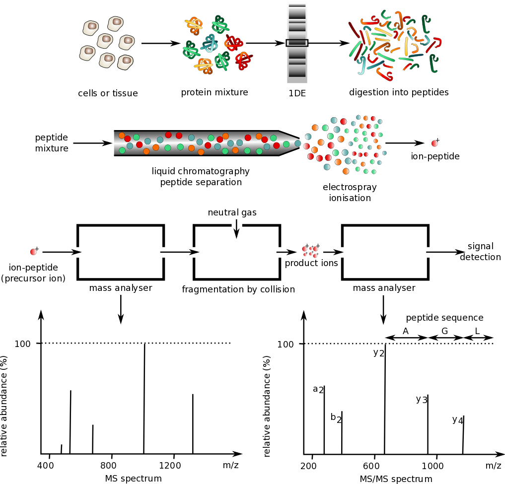
Protein mixtures are prepared from cell culture or tissue samples and separated by gel electrophoresis. Single proteins are isolated and digested using trypsin to produce a peptide mixture. Peptides are separated by liquid chromatography and analyzed by mass spectrometry

3D Structural Determination

The 3D structure of a protein can be determined in four main ways: X-ray crystallography, multidimensional NMR, cryoelectron microscopy, and computer modeling using artificial intelligence and machine learning.

X-Ray Crystallography

In this technique, proteins are induced to form solid crystals in which the individual molecules pack in a well-defined crystal lattice. X-rays are aimed at the crystals. The X-rays are scattered off the crystal and collected by a detector. The scattered X-rays undergo constructive and destructive interference (as water waves do), forming a diffraction pattern. The crystal's spacing and types of atoms determine the diffraction pattern. Hence, from a given 3D structure, a specific diffraction pattern is formed. Using sophisticated mathematics (Fourier Transformations), the diffraction pattern can be converted back into the 3D structure of the object —in this case, the protein's atoms.

PHET Simulation - Diffraction

Constructive and destructive interference and the formation of a "diffraction" pattern can be readily visualized in two PHET simulations. Follow the instructions below.

Simulation 1: Slits

• Select Slits to open the simulation and select these choices in order:
• Type of wave: pick one that looks like a bullet
• Frequency (middle green)
• Amplitude: max
• Check Screen
• Choose 2 Slits
• Slit width 200
• Slit separation 400
• Click the Green button.

You will see light/dark patterns moving toward the screen. The light zones arise from constructive interference and dark from destructive interference of the two waves as they emerge from the slits.

Simulation 2: Diffraction

Now, look at the diffraction pattern from light moving through simple and more complex openings and interacting with an object using the PHET animation and the step below.

• First, refresh the browser window.
• Select Diffraction to open the simulation and select these choices in order.
• Pick 450 nm wavelength.
• Choose in succession the four vertical icons (circle, square, circle/square, array of circles, person).
• Observe the diffraction patterns as you change the slit size.

X-ray scattering can also be viewed as light "reflecting" from a series of planes formed by atoms in the crystal, with the planes separated by specific distances (in the Angstrom range). The x-rays that are "reflected" from innumerable planes recombine constructively and destructively to form a diffraction pattern. X rays are used since the size of the "slits", and the distance between these "reflective" planes, must be comparable to the wavelength of the incident light, which for x-rays is 0.5 – 2.5 Å.

A diffraction pattern is mathematically decoded to form an electron density map, since electrons scatter X-rays. Hydrogen atoms don't appear in X-ray crystal structures because they lack sufficient electrons to serve as effective scattering centers. Computer programs are used to fit the electron density map to a 3D arrangement of atoms separated by characteristic bond distances corresponding to the functional groups and side chains found in proteins. The quality/amount of crystals helps determine the quality of the diffraction pattern and the resulting structure. X-ray crystallographers define quality in terms of resolution. A resolution of 5 Å - 10 Å can reveal the structure of polypeptide chains, 3 Å - 4 Å of groups of atoms, and 1 Å - 1.5 Å of individual atoms.

Figure \(\PageIndex{18}\) shows the process from crystal to model.

Figure \(\PageIndex{18}\): Overview of structure determination by mass spectrometry. Thomas Splettstoesser (www.scistyle.com), CC BY-SA 3.0 <https://creativecommons.org/licenses/by-sa/3.0>, via Wikimedia Commons

 

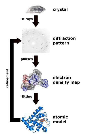
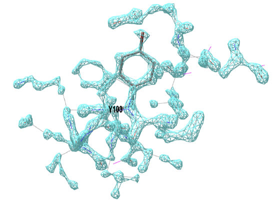
 Figure \(\PageIndex{19}\) below shows the electron density map around tyrosine 103 from myoglobin from crystal structures at two different resolutions (left, 1a6m, 1.0 Å resolution and right, 108m, 2.7 Å resolution).

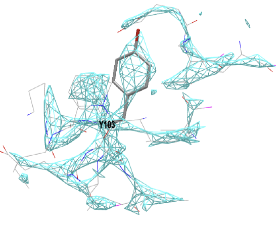Figure \(\PageIndex{19}\):  Electron density map around tyrosine 103 from myoglobin from crystal structures at two different resolutions (left, 1a6m, 1.0 Å resolution and right, 108m, 2.7 Å resolution).  Click on the images to see full iCn3D models showing the electron density map around the Y103. (Choice of Y103 from https://pdb101.rcsb.org/learn/guide-...ata/resolution)

This figure shows 2Fo-Fc electron density maps, which use the observed diffraction data (Fo) and the diffraction data calculated from the atomic model (Fc). Proteopedia has an excellent description of electron density maps.  

Not all proteins can be readily crystallized. The process is, in many ways, an art as much as it is a science. Membrane proteins fall into this category.

Nuclear Magnetic Resonance (NMR)

Many readers have probably performed ¹H-NMR on small molecules in introductory and organic chemistry labs. Interpreting spectra of molecules with many hydrogen atoms in straight and branched chains, in rings, and in functional groups is not simple. Imagine doing that to determine the structure of a small protein with 1000s of hydrogen atoms! The spectrum would be essentially indecipherable. Luckily, multi-dimensional NMR techniques have allowed the solution (not crystal) structure of small proteins to be determined. These methods are outside of the scope of this book. For those interested in more detail, read A Brief Introduction to NMR Spectroscopy of Proteins by Poulsen.

Let's briefly introduce a 2D NMR peak for a simple molecule, ethyl acetate. The 1D ¹H-NMR spectrum for the molecule is shown in Figure \(\PageIndex{20}\).

Figure \(\PageIndex{20}\): 1D ¹H-NMR spectrum of ethylacetate

Now, let's show a simulated 2D COSY spectrum of the same molecule. The image and explanation below are adapted from Structure & Reactivity in Organic, Biological, and Inorganic Chemistry by Chris Schaller, licensed under a Creative Commons Attribution-NonCommercial 3.0 Unported License. Structure and Reactivity

In homonuclear correlation spectroscopy (COSY), we can look for hydrogens that are coupled to each other. In ethyl acetate, it's pretty clear where they are. There is a quartet and a triplet; the hydrogens corresponding to those two peaks are probably beside each other in the structure. The COSY spectrum takes that ¹H spectrum and spreads it into two dimensions. Instead of being displayed as a row of peaks, the peaks are spread out into a 2D array. Figure \(\PageIndex{21}\) shows an annotated simulated COSY spectrum. The peaks are displayed along one axis, and the same peaks are displayed along the other.

Figure \(\PageIndex{21}\): Annotated simulated COSY spectrum of ethylacetate

What does it mean to be coupled? It means that magnetic information is transmitted between the atoms. How can we tell? Essentially, we can send a pulse of electromagnetic radiation into one set of hydrogen atoms and look for a response elsewhere. Of course, if we send a pulse of radio waves at a frequency that a particular hydrogen will absorb, we will see a response in that hydrogen itself. That's why we see the peaks on the diagonal (dotted line). The peaks along the diagonal in the spectra (1.26, 1.26; 2.04, 2.04; 4.12, 4.12) don't provide any new information, since they are the main peaks in the 1D NMR.

However, we also see responses from other hydrogen atoms magnetically linked to the original one. They give the peaks (shown as purple circles) that do not appear along the diagonal. Those peaks indicate which hydrogens are coupled to which other hydrogens. The hydrogens at 1.26 ppm are coupled to the ones at 4.12 ppm, giving a "cross-peak" at (1.26, 4.12). There is also a cross-peak at (4.12, 1.26) because that relationship goes both ways.

This coupling should make sense because the protons that give the signals at 4.12 (-O-CH₂-CH₃) and 1.26 (-CH₂-CH₃) are on adjacent carbons and split each other's signals, as seen in the 1D NMR. This example shows how we can identify which protons in a 2D NMR spectrum are coupled through 3 bonds (H-C-C-H), a critical piece of information for determining protein structures by NMR.

Variants of 2D NMR are also used in protein structure. They use NMR-active nuclei in addition to ¹H, including ¹³C (natural abundance 1%) and ¹⁵N (natural abundance 0.37%). Given these low abundances, proteins for NMR structure determination are often purified in cells grown in media enriched in ¹³C and ¹⁵N precursors.

HMBC (Heteronuclear Multiple Bond Correlation) and HMQC (Heteronuclear Multiple Quantum Coherence): Just as COSY spectra show which protons are coupled to each other, HMBC (and the related HMQC) give information about the relative relationships between protons and carbons in a structure. In an HMQC spectrum, a ¹³C spectrum is displayed on one axis and a ¹H spectrum on the other. Cross-peaks show which proton is attached to which carbon. COSY spectra show a 3-bond coupling (from H-C-C-H), whereas HMQC shows a 1-bond coupling (just C-H).

Nuclear Overhauser Effect (NOE) Spectroscopy (NOESY): This technique shows through-space interactions within the molecule rather than the through-bond interactions in COSY and HMBC/HMBQ. This method is especially useful for determining a molecule's stereochemical relationships. In two stereoisomers, all atoms are connected in the same order by the same bonds. A COSY or an HMBC spectrum couldn't distinguish between these isomers.

HNCA: This is an example of 3D NMR. It shows a correlation between an amide proton, the amide nitrogen to which it is attached, and the carbons attached to the amide nitrogen. HNCA data are viewed in slices, where you examine one nitrogen at a time. One axis shows the shift of the proton attached to that nitrogen, and the other axis shows the shifts of the carbons attached to the nitrogen. The abbreviation HNCA comes from the pathway for transferring magnetization (amide H to amide N, then to the attached C-alpha).  

NMR structures in the Protein Data Bank consist of many slightly different structures. This arises from the dynamic behavior of the proteins in water, compared to when the structure is determined from a crystal. Comparative analyses between crystal and NMR structures show that secondary structures are equally accurate, that loops in NMR structures are probably too flexible, and that loops in protein, often on the surface, are too rigid, which makes sense given the packing restraints with a crystal lattice.

Cryo-electron Microscopy

Cryogenic-electron microscopy (cryo-EM) has recently emerged as a powerful structural biology technique that delivers high-resolution density maps of macromolecular structures. Figure \(\PageIndex{22}\) shows a cryo-EM and structure determined from it.

Figure \(\PageIndex{22}\): Cryo-Electron Microscopy. (a) the Scottish Centrel for Macromolecular Imaging JEOL CryoARM 300. (b) High-resolution 2.2-Å resolution structure of lumazine synthase. Bhella, D. (2019) Biophysical Reviews 11:515-519. Creative Commons Attribution 4.0 International License (http://creativecommons.org/licenses/by/4.0/)

Resolutions approaching 1.5 Å are now possible, and maps in the 1–4-Å range inform the construction of atomistic models with high confidence. This new capacity for investigators to determine macromolecular structures at high resolution and without the need to form crystals has led to an explosion of interest in adopting cryo-EM.

Protein suspensions are frozen on 3-mm-diameter transmission-electron microscope (TEM) support grids made from a conductive material (e.g., Cu or Au) that are coated with a carbon film with a regular array of perforations 1–2 μm in diameter. A total of 3–5 μl of sample is loaded onto the grid, which is then immediately blotted with filter paper to create a film of buffer/protein on the grid that, when frozen, will be thin enough for the electron beam to penetrate. Optimizing ice thickness is a vital step in sample preparation, as thicker ice layers increase the likelihood that an incident electron will undergo multiple scattering, thereby reducing image quality. In the case of extreme ice thickness, the electron beam does not penetrate at all. After blotting, the grid is rapidly plunged into a bath of liquid ethane—a very effective cryogen that freezes water rapidly enough to prevent ice crystal formation. Forming a vitreous ice layer is the fundamental step in cryo-EM and preserves the target in a near-native state. The resulting vitreous ice layer with suspended protein molecules must then remain close to liquid nitrogen temperature (− 196 °C) during storage and TEM imaging to prevent phase changes to other types of ice that are not amenable to high-quality imaging and preservation of protein structure.

Figure \(\PageIndex{23}\) summarizes the process and single particle structure determination.

 

Figure \(\PageIndex{23}\):  Principle of cryo-EM and single-particle reconstruction.  Agirrezabala, X., Frank, J., 2010. From DNA to proteins via the ribosome: Structural insights into the workings of the translation machinery. Human Genomics 4, 226. https://doi.org/10.1186/1479-7364-4-4-226.  CC BY 4.0

The figure above shows the cryoEM structure-determination process for ribosomes.  When frozen, they are found in random orientations embedded in a thin layer of ice. Exposure to a low-dose electron beam in the transmission electron microscope produces a projection image (i.e., the electron micrograph). A typical electron micrograph shows E. coli ribosomes as low-contrast single particles on a noisy background. After the orientations of the particles have been determined, usually by matching them to a reference using computer algorithms, they are used to reconstruct a density map using back-projection or a similar reconstruction algorithm. This density map is segmented into components (subunits, ligands), and these components are displayed in different colors in a surface representation (bottom panel; small and large subunits are shown in yellow and blue, respectively). A- and P-site tRNAs are colored red, pink, and green, respectively.

Given the increasing popularity of this technique, we present Figure \(\PageIndex{24}\) below, which shows another representation of the end-point of a higher-resolution 3D model.

Figure \(\PageIndex{24}\): A schematic of the single-particle reconstruction cryoEM pipeline. Hey Tony et al., 2020. Machine learning and big scientific data. Phil. Trans. R. Soc. A.3782019005420190054.  http://doi.org/10.1098/rsta.2019.0054.  Creative Commons Attribution License http://creativecommons.org/licenses/by/4.0/

Motion occurs when the beam strikes the ice dome, where the single structure is found. Motion pictures are captured with fast detectors, and computers are used to compensate for motion, which reduces the resolution of the structure. In addition, as X-rays damage molecules, so can electron beams. Earlier frames in the movie show less damage. The beam's motion and damage effects can now be corrected to increase the resolution.

Here is a YouTube video from PDB 101 that describes the technique.

Methods for determining atomic structure.  PDB-101: Educational resources supporting molecular explorations through biology and medicine. Christine Zardecki, Shuchismita Dutta, David S. Goodsell, Robert Lowe, Maria Voigt, Stephen K. Burley. (2022) Protein Science 31: 129-140 https://doi.org/10.1002/pro.4200.   CC By 4.0 license.  

Prediction of Protein Structure and Protein Function

A new chapter section, 4.14: Predicting Structure from Sequence and Sequence from Structure/Function (New 10/24), has been created to reorganize material on predicting protein structure from sequence and the reverse problem: predicting sequence from protein structure (for designer proteins) and from protein function.  

Comparisons of 3D Structure Determination Methods

Obtaining a pure, highly concentrated (mM) protein sample is a major bottleneck for X-ray crystallography and NMR. The high concentration is required because both techniques are insensitive to single-molecule analysis, and a large population of a particular protein is required to overcome the signal-to-noise barrier. Similarly, the sample needs to be very homogeneous, so protein purification is necessary at some point. Cryo-EM requires considerably less protein than the other two methods, but still a lot by any standard. Typically, Cryo-EM requires preparations at a concentration of 1 mg/ml in a volume of at least 50 μl. In contrast, crystal formation might require 500 μl of protein at 5 -10 mg/ml concentration. Cryo-Em requires the protein to be prepared in a low-salt buffer solution with minimal additives to ensure good freezing and image contrast.

Recombinant protein production using E. coli is the method of choice when large quantities of protein are required. This process involves cloning the gene (often cDNA) encoding the protein of interest into a suitable inducible vector, transforming the vector into an E. coli host, and growing the culture in a rich medium. The bacterial host will multiply during a growth phase, after which it is induced to express the protein of interest. If all goes well, the protein will be soluble and expressed at high levels. Unfortunately, this process is easier said than done. Many eukaryotic proteins do not express well in prokaryotic hosts, and modifications are needed to optimize the bacterial host, codon usage, media, etc., to obtain a decent yield of recombinant protein.

Additionally, expressed proteins are often found as insoluble inclusion bodies and require high concentrations (2M to 8M) of denaturants such as urea or guanidine hydrochloride to solubilize them, followed by stepwise dialysis into an appropriate buffer to refold them. Alternatively, eukaryotic organisms such as S. cerevisiae (yeast), insect, and mammalian cell lines can be used, especially if post-translational modifications are studied. However, yield decreases and overall costs increase are common with these organisms.

Protein production is difficult for ¹⁵N- and ¹³C- NMR because proteins must be labeled with these isotopes. Only these isotopes have nuclei with + ½ and -½ spin states, which enable the energy transitions required for a radiofrequency NMR signal.  Of course, ¹H also has ½ spin states but is highly abundant.

Protein stability is an issue for both crystallography and NMR. Once a protein has been expressed, purified, and concentrated, it must maintain its structural integrity for the experiments. In crystallography, a protein sample is placed in various solutions (often high in polyethylene glycol) that promote crystallization. Crystallization conditions are tested in a high-throughput 96-well screening plate format, and any hits are further optimized using a larger volume of the corresponding solution. While a crystallization condition may eventually be found, the process can take anywhere from a few days to a year or two, making it the rate-limiting step for protein crystallographers. During this time, the protein must stay in solution and maintain its structure to produce a high-quality crystal, a condition that may not be met.

Similarly, a stable, highly concentrated protein sample is required to perform more advanced NMR experiments. These experiments require days or even weeks to run, during which the solution's homogeneity is key to obtaining high-quality spectra. Should the protein unfold or precipitate from solution during an experiment, the resulting chemical change would either not produce a signal or one that could not be used to determine structure/dynamics.

Working with frozen-hydrated specimens for Cryo-EM brings many challenges for manipulations and imaging. Exposure to atmospheric water vapor rapidly leads to frost buildup on the grid when handling cryo-EM grids for loading into the microscope. Under the TEM, these ice crystals on the grid surface appear as huge boulders that completely block the electron beam. Thus, grids are kept under liquid nitrogen whenever possible to minimize frost contamination. Problems with ice conditions are common—insufficient rapid freezing leads to hexagonal ice, while devitrification occurs when samples warm up, forming cubic ice. Various degrees of contamination may occur, and frosting at atmospheric pressure can cause the aforementioned ice crystal deposition. In contrast, contamination within the column or under low-vacuum conditions results in a more subtle artifact.

One of the hallmarks of protein crystallography is that size does not matter. Whether working with a 25 kDa monomeric protein or a 900 kDa multimeric complex, its structure can be determined if it can be crystallized and produce a high-resolution diffraction pattern. This is because, once in crystal form, a protein is in a more-or-less static conformation that can yield a single structural model in X-ray crystallography. Cryo-EM is similar in this regard. Very large structures, including massive nucleoprotein complexes, such as the ribosome, can be elucidated using Cryo-EM. The same cannot be said for NMR.

In NMR, the protein is in a soluble state and, therefore, in constant movement. The molecular tumbling rate is the most important movement governing spectral quality. The tumbling rate decreases significantly for proteins larger than 40 kDa, increasing the transverse relaxation rate (T₂). This results in a weaker, rapidly decaying NMR signal, leading to peak broadening and spectral overlap.

One of the major advantages of NMR is its ability to record small and large-scale protein dynamics, which is suppressed when a protein is crystallized. Although a crystallized protein may exhibit some motion within the lattice, these motions manifest as static or dynamic disorder, resulting in two different conformations of a particular region and, in the latter case, an averaged electron density. In general, crystallization may restrict a protein’s natural flexibility and motions. Cryo-EM suffers from this same limitation as samples are frozen and immobile. However, cryo-EM can capture a snapshot of the native structure as freezing is instantaneous and does not require crystal lattice formation.

Crystallography, however, is not left out of dynamic structural analysis. Time-resolved crystallography can monitor protein structural changes upon ligand addition or environmental perturbations. Because all protein crystals are highly hydrated, they can serve as crucibles for some biochemical reactions. The crystal is typically soaked in a solution containing the ligand of interest to initiate the biochemical reaction, then quickly placed on the beamline, and the diffraction pattern is obtained. This can be performed multiple times if necessary to obtain a variety of structural intermediates. The process requires many things to go right: the protein cannot become disordered, the crystal cannot crack during soaking, and a high-powered synchrotron is required to collect high-quality diffraction data over short exposure times.

In the end, protein X-ray crystallography, cryo-EM, and NMR spectroscopy are not mutually exclusive techniques; one can easily fill in where the other falls short. In analyzing NMR dynamics experiments, for example, one can greatly benefit from existing crystal structure data or cryo-EM data onto which the NMR structural data can be superimposed. Similarly, NMR structure data can supplement cryo-EM or crystal structures with additional information on the protein's dynamics, binding interactions, and conformational changes in solution.

 

Molecular Dynamics Simulations

Introduction to Molecular Mechanics and Molecular Dynamics

Molecular modeling and computational chemistry are important parts of modern biochemistry.  Models display, in a meaningful and instructive way, the large amounts of data generated when X-ray crystallography and NMR are used to determine the structures of large biological molecules and complexes.   Remember, however, that primary X-ray crystallographic data (in the form of electron density maps) are just that; they must be interpreted like any other type of data.  Structures must be refined and energy minimized to produce more realistic structures (without van der Waals overlap or missing atoms, for example).  In addition, atoms within any molecule are not static but move as bonds vibrate, angles bend, etc.  This implies that large biomolecules can adopt many possible conformations of varying energy.  For proteins, some of these conformations might center on an average conformation at a local or global energy minimum, separated by activation energy barriers. 

In contrast, small molecules whose structures can be minimized using ab initio or semi-empirical quantum mechanics (e.g., Spartan), large molecular structures (such as DNA, RNA, proteins, and their complexes) must be minimized using molecular mechanics based on Newton's laws.  Atoms are treated as masses and bonds as springs with appropriate force constants.  A force field containing all the relevant parameters for a given atom (for example, sp³, sp², sp² aromatic, and sp C) and bond types is used to solve energy equations that sum all energies over all atoms and bonds in the molecule.  These energies include interactions among bonded atoms (stretching, bending, torsion, wagging) and those among nonbonded atoms (electrostatic and van der Waals).   In minimization calculations, the positions of atoms within a molecule are systematically or randomly moved, and the energy is recalculated to find a lower energy state and, hence, a more stable molecule.  Minimization calculations can not probe all conformational space or easily move a structure from a local minimum to a global minimum if a large energy barrier separates the two.  Energy minimization is usually performed in the absence of a solvent.  Common force fields used for macromolecules are CHARMM, AMBER, and GROMOS.  Parameters for specific atom types in a given bond include atomic mass, van der Waals radius, partial charge for atoms (from quantum mechanics), bond length (from electron diffraction data), angles, and force constants for bonds (modeled as springs, obtained from IR).  These parameters are derived from experiments and theoretical (usually quantum mechanical) calculations on small organic molecules.  A potential energy equation comprising terms from bond stretching, angle bending, and torsional angle changes (bonded interactions), as well as electrostatic and van der Waals interactions (nonbonded), is then solved (described below).

Molecular dynamics aims to simulate the actual changes in a molecule over time after an energy input (e.g., heat application at a higher temperature) is added to a molecule at equilibrium.  The structure is placed in a "bath" of thousands of water molecules to make the simulation realistic.  As is described below, if the energies of atoms in a large molecule are known, the forces acting on those atoms can be deduced.  From Newton's Second Law (F = ma), the velocity, or change in position, of an atom in the structure over time can be determined.  Suppose the dynamic simulation can be run for a long enough time. In that case, alternate conformations (perhaps those centered around a global minimum and those nearby in energy space—local minima) may be sampled.  By determining what fraction of the simulated conformations resemble the two alternative conformations, the ΔG for the interconversion of the two states can be calculated.  As you can imagine, these calculations require substantial computer time.  They give very important information. However, protein conformational changes are often, if not always, associated with binding a biological molecule to a binding partner.  In silico experiments offer important clues and support for results obtained using other study methods.  

Molecular mechanics (MM) and molecular dynamics (MD) have become powerful tools for analyzing and predicting the properties of complex biological structures.  The Nobel Prize in Chemistry in 2013 was awarded to Martin Karplus, Michael Levitt, and Arieh Warshel "for the development of multiscale models for complex chemical systems". Karplus, in particular, developed much of the present basis for MD simulations.

Energy (E), Force (F), and Motion

Considering the relationship between force and energy helps make the energy equations for the individual components more understandable.  You have studied two general force equations in introductory chemistry and physics courses.  Coulomb’s Law describes the electrostatic force of attraction, F_C, between two charges, q₁ and q₂, separated by a distance r.

\begin{equation}
F_C=k \frac{q_1 q_2}{r^2}
\end{equation}

The other is Hooke’s Law, which describes the restorative force on a mass connected to a spring on stretching or compression of the spring.

\begin{equation}
F=-k x
\end{equation}

where x is the spring's displacement from an equilibrium (at rest) position. 

Our first interest is understanding how these equations might lead to equations describing the potential energy of a two-charge system or a compressed or stretched spring.  We can best understand this by considering a simple example: a ball placed at various locations on a hill.  If placed on a flat surface at the top and bottom of the hill, no net force is acting on the ball (F_net = 0), so it will not move.  If placed at various locations on the downslope, it will experience a net downward force, shown qualitatively in Figure \(\PageIndex{25}\) below. 

Figure \(\PageIndex{25}\): Potential Energy vs r for a ball on a hill

Astute observers will note that the magnitude of the force vector is proportional to the slope.  From this simplistic approach, we come to the following equation relating F to E:

\begin{equation}
F=-\frac{d E}{d r}
\end{equation}

The minus sign is required since the force is downward, but the energy increases upward.

This simplified approach can be extended into three dimensions to give the following equation (which will have meaning to those with an advanced calculus background), where F is the negative gradient of the potential energy:

\begin{equation}
F=-\left(\frac{\partial}{\partial x}+\frac{\partial}{\partial y}+\frac{\partial}{\partial z}\right) E=-\nabla E
\end{equation}

Applying the 1D equation to Hooke’s Law gives

\begin{equation}
\begin{aligned}
& d E=-F d r=-k x d x \\
& \int d E=-k \int x d x
\end{aligned}
\end{equation}

which gives

\begin{equation}
E=\frac{k x^2}{2}
\end{equation}

This gives a parabolic graph of E vs displacement. Figure \(\PageIndex{26}\) below shows an interactive PHET simulation of Hooke's Law.  Click Energy and then select Energy to see the parabolic plot.  Change the force constant to alter the "steepness" of the resulting parabolic curve.

Figure \(\PageIndex{26}\): PHET simulation of Hooke's Law.  https://phet.colorado.edu/en/simulations/hookes-law

The same approach can be applied to Coulomb's Law.  Notice that the result equation for E results in increasingly negative values as r gets smaller, only when q1 and q2 have opposite charges. 
 

\begin{equation}
\begin{aligned}
& d E=-F d r=-k \frac{q_1 q_2}{r^2} d r \\
& \int d E=-k q_1 q_2 \int r^{-2} d r
\end{aligned}
\end{equation}

gives

\begin{equation}
E=\frac{k q_1 q_2}{r}
\end{equation}

A graph of E vs r for both attractive and repulsive interactions is shown in Figure \(\PageIndex{27}\) below.

Figure \(\PageIndex{27}\): E vs r for both attractive and repulsive interactions

 

Molecular Mechanics

Note: The following review is based on an NIH Guide to Molecular Modeling (1996), which, to the best of our knowledge, was removed from the web.  

Molecular mechanics uses Newtonian mechanics to calculate the energy of atoms in large molecules, such as proteins.  It assumes that nuclei and electrons are single particles with radii and calculated charges.  Bonds are treated as springs connecting atoms.  Energies are calculated classically (not with quantum mechanics).  Parameters, many based on quantum mechanical calculations of small molecules, are assigned to all bonds, angles, dihedrals, etc.  Interactions are bonded (local) and nonbonded.

Bonded interactions involve atoms connected by one bond (bond stretch), two bonds (angle bending), and three bonds (dihedral angle change). These three types of bonded interactions are shown with black arrows on the right-hand side of Figure \(\PageIndex{28}\) below.

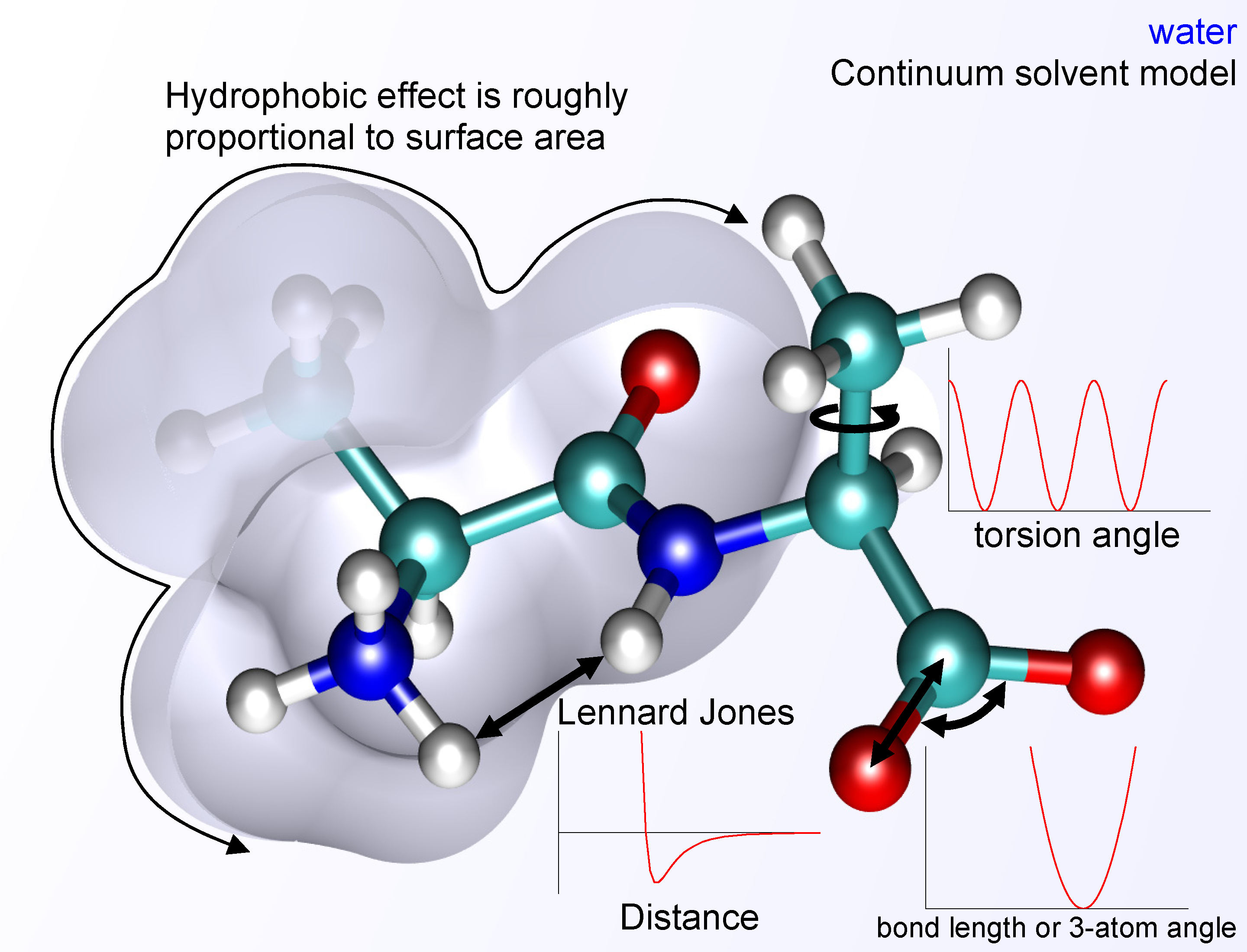
Figure \(\PageIndex{28}\):  Bonded and Nonbonded Interactions in Proteins.  Force field (chemistry). (2023, July 15). In Wikipedia. https://en.wikipedia.org/wiki/Force_field_(chemistry).  CC BY-SA 3.0

Non-bonded atoms (greater than two bonds apart) interact through induced dipole-induced dipole interactions (one example of which is steric repulsions) and electrostatic attraction/repulsion. The double black arrow labeled Lennard-Jones in the above figure shows an example of a nonbonded interaction.

All energy terms from these interactions are summed to give the energy of a given conformation.  The energy should be considered relative to that of other conformations. Here is the basic energy equation for all of these energy terms:

\begin{equation}
\text { Energy }(\mathrm{E})=\mathrm{E}_{\text {Stretch }}+\mathrm{E}_{\text {Bending }}+\mathrm{E}_{\text {Torsion }}+\mathrm{E}_{\text {Non-bonded Interactions }}
\end{equation}

The "force field" consists of the energy equations and the parameters for each energy term. Many different commercially available force fields exist.

Bonded Interaction Energies

The mathematical form of the energy terms varies from force field to force field. The more common forms will be described.

Stretching (Vibrational) Energy

\begin{equation}
\mathrm{E}_{\text {stretch }}=\Sigma_{\text {bonds }} \mathrm{k}_{\mathrm{b}}\left(r-\mathrm{r}_{\mathrm{o}}\right)^2
\end{equation}

Figure \(\PageIndex{29}\) illustrates bond stretching or vibration 

Figure \(\PageIndex{29}\): Bond stretching or vibration 

The stretching energy equation is based on Hook's law. The k_b parameter defines the bond spring's stiffness.  R₀ is the equilibrium distance between the two atoms.   It should make sense that deviations from the equilibrium length would be associated with higher energy.  The E vs. r curve is a parabola, as shown in Figure \(\PageIndex{30}\) below for a system with the lowest energy at r=6.

Figure \(\PageIndex{30}\): Energy vs r (r₀=6) for bond stretching (vibration)

Only small changes in r are allowed, as too large an r value would lead to bond breaking.

Bending Energy

\begin{equation}
\mathrm{E}_{\text {bending }}=\Sigma_{\text {angles }} k_{\Theta}\left(\Theta-\Theta_0\right)^2
\end{equation}

Figure \(\PageIndex{31}\) illustrates bond bending

 

Figure \(\PageIndex{31}\): Bond bending

The bending energy equation is also based on Hooke's law. The kΘ parameter controls the stiffness of the angle spring, while the Θ₀  is the equilibrium angle. As above, the graph of E vs theta is expected to be a parabola as shown in Figure \(\PageIndex{32}\) below for a system when the lowest energy is at θ=45

Figure \(\PageIndex{32}\): E_bending vs r when lowest energy is at θ=45. 

Torsion Energy

\begin{equation}
E_{\text {torsion }}=\Sigma_{\text {torsions }} A[1+\cos (\text { ntau }-\Theta)]
\end{equation}

Figure \(\PageIndex{33}\) illustrates torsion angle rotation

 

Figure \(\PageIndex{33}\): Torsion angle rotation

The torsion energy is modeled by a periodic function, much as you have seen with energy plots associated with Newman projections sighting down the central C-C bond in butane.  Figure \(\PageIndex{34}\) below shows two different torsion energy functions.

Figure \(\PageIndex{34}\): Torsion energy vs tau for A=1, n=1, phi=0 (blue) and A=1, n=2,phi=90 (orange).

 

Non-Bonded Interaction Energy

The non-bonded energy is calculated for all possible pairs of nonbonded atoms, i and j:

E_nonbonding = Σ_i Σ_j [ -B_ij/r_ij⁶ +A _ij/r_ij¹² ] + Σ_i Σ_j (q_i q_j) / r_ij 

\begin{equation}
E_{\text {nonbonding }}=\Sigma_i \Sigma_j\left[-B_{i j} / r_{i j}^6+A_{i j} / r_{i j}^{12}\right]+\Sigma_i \Sigma_j\left(q_i q_j\right) / r_{i j} \mid
\end{equation}

The first term represents van der Waals interactions, while the second represents Coloumbic electrostatic interactions.  Figure \(\PageIndex{35}\) illustrated nonbonded interactions.

Figure \(\PageIndex{35}\): Nonbonded interactions

You should remember that induced dipole-induced dipole interactions are short-range and occur among all atoms. The 6-12 energy equation, based on the Lennard-Jones potential, shows a negative (attractive) term proportional to -1/r⁶ and a repulsive term proportional to +1/r¹².  Figure \(\PageIndex{36}\) below shows a graph of the attractive, repulsive, and summation of the energy terms in the Lennard-Jones potential. 

 

Figure \(\PageIndex{36}\): Lennard-Jones potential vs r

The A and B parameters control the depth and position (interatomic distance) of the potential energy for a pair of non-bonded interacting atoms (e.g., C:C and O:C). In effect, A determines the degree of stickiness of the van der Waals attraction, and B determines the degree of hardness of the atoms (e.g., marshmallow-like, billiard ball-like, etc.).

The B parameter is related to the "stickiness" of the interactions and the polarization of the atoms. B can be obtained from atomic polarizability measurements or calculated using quantum mechanics. The A parameter is empirically derived to fit nonbonded contacts between atoms in crystal structures. 

Summary Interactions

Some programs assign charges using rules or templates, especially for macromolecules. The torsional potential is calibrated to a particular charge calculation method in some force fields. Using a different method can invalidate the force-field consistency.  An additional bonded interaction term, improper dihedrals, is sometimes added, as illustrated below.  The following equation gives the potential for that:

E_improper = Σ_angles kω (ω - ω_o)² 

\begin{equation}
E_{\text {improper }}=\Sigma \text { angles } k \omega\left(\omega-\omega_0\right)^2
\end{equation}

 

Molecular Dynamics

This section comes directly from the NIH tutorial:

"In the broadest sense, MD is concerned with molecular motion. Motion is inherent to all chemical processes. Simple vibrations, like bond stretching and angle bending, give rise to IR spectra. Chemical reactions, hormone-receptor binding, and other complex processes are associated with many intra- and intermolecular motions.

Thermodynamics describes the driving force for chemical processes, while kinetics describes the mechanism by which they occur. Thermodynamics governs the energetic relationships between different chemical states, while kinetics describes the sequence and rates of events that occur as molecules transform between their various possible states.

Molecular dynamics studies usually focus on conformational transitions and local vibrations. MD alters the intermolecular degrees of freedom step-wise, analogous to energy minimization. The individual steps in energy minimization aim only to establish a downhill direction toward a minimum. On the other hand, the steps in MD meaningfully represent the changes in atomic position, ri, over time (i.e., velocity).

Newton's equation (F_i = m_iaⁱ) is used in the MD formalism to simulate atomic motion. As Newton's equation states, the rate and direction of motion (velocity) are governed by the forces that the system's atoms exert on one another. In practice, the atoms are assigned initial velocities that satisfy the total kinetic energy of the system, which, in turn, is determined by the desired simulation temperature. This is done by slowly heating the system (initially at absolute zero) and allowing the energy to equilibrate among the constituent atoms. The basic ingredients of MD are the calculation of the force on each atom and, from that information, the position of each atom through a specified time (typically on the order of picoseconds = 10^-12 seconds).

The force on an atom can be calculated from the change in energy between its current position and its position a small distance away. This can be recognized as the derivative of the energy with respect to the change in the atom's position: -dE/dr_i = F_i.

Energies can be calculated using either MM or quantum mechanics methods. MM energies are limited to applications that do not involve drastic changes in electronic structure, such as bond-making or breaking. Quantum mechanical energies can be used to study dynamic processes involving chemical changes. The latter technique is extremely novel and limited in availability.

Knowledge of atomic forces and masses can then be used to determine the positions of each atom at a series of extremely small time steps (on the order of femtoseconds). A trajectory is the resulting series of snapshots of structural changes over time. The use of this method to compute trajectories can be more easily seen when Newton's equation is expressed in the following form

-dE/dr_i = m_ia= md²r_i/dt² 

\begin{equation}
-d E / d r_i=m_i a=m d^2 r_i / d t^2
\end{equation}

In practice, trajectories are not obtained directly from Newton's equation because there is no analytical solution. First, the atomic accelerations are computed from the forces and masses acting on each atom. The velocities are next calculated from the accelerations based on the following relationship:
a_i = dv_i/dt. Lastly, the positions are calculated from the velocities: v_i = dr_i/dt. A trajectory between two states can be subdivided into sub-states separated by a small time step, delta t (e.g., 1 femtosecond).

The initial atomic positions at time t are used to predict the atomic positions at time t = delta t. The positions at t = delta t are used to predict the positions at t = 2Δt, and so on.

The leapfrog method is a common numerical method for calculating trajectories from Newton's equations. The method derives its name from the fact that velocity and position information alternate at ½-time-step intervals.  MD has no defined termination point other than the time that can be practically covered.

Figure \(\PageIndex{37}\) below shows a 0.5 ns molecular dynamics simulation of sperm whale myoglobin, a muscle protein that binds O₂ at a macrocyclic ligand called heme.  The heme and oxygen were not included in the simulation.  The protein (molecular weight 17,331), consist of 8 alpha helices (red) connected by random coils.  The backbone and side chains are shown in green sticks.  

Figure \(\PageIndex{37}\):  A 0.5 ns molecular dynamics simulation of sperm whale myoglobin. 

The simulation was performed in GROMACS using NeuroApp.  The input PDB files for the simulations were first processed using Charmm-GUI.  The output simulation files (input_protein and md_center.xtc from the output folder) from the Gromacs simulation were opened in Pymol and processed to make the animations shown above (File, Export Movie, as PNG, then animated GIF in Adobe Photoshop). Abraham, J. M. et al., GROMACS: High-performance molecular simulations through multi-level parallelism from laptops to supercomputers, https://www.sciencedirect.com/, September 2015, https://doi.org/10.1016/j.softx.2015.06.001. Neurosnap Inc. - Computational Biology Platform for Research. Wilmington, DE, 2022. https://neurosnap.ai/.

A molecular dynamics simulation of a small protein module (NTL9) folding is shown below.

 

MD simulations can be used to obtain theoretical values for ΔG and Keq values for conformational changes, binding of small ligands, and changes in protonation states for side chains.   This process is based on the idea that the conformations sampled in silico MD simulations reflect those found in vitro (i.e., they are part of the thermodynamically expected and accessible conformations of the molecules during normal conformational shifts).  This is called the Ergodic Hypothesis.  Given the short time scales of MD simulations (limited by computer power), this hypothesis can't apply to dynamic results unless the sample conformations are close in energy, with no large activation energy barrier between them.     If it is, then the following equation could apply:

\begin{equation}
\begin{aligned}
& \Delta G^0=-R T \ln K_{\text {eq }} \\
& \Delta G^0=-R T \ln P_2 / P_1=-R T \operatorname{ln} f_2 / f_1
\end{aligned}
\end{equation}

where

P_n is the probability of being in a given state, and f_n is the fraction in a given state.

You will note that none of the potential energy functions use quantum mechanical parameters.  This is due, in part, to the complexity of the systems studied.   This is beginning to change as more effort is devoted to understanding the quantum mechanical aspects of complex bonded systems.  New advances in even simple systems can illustrate this point.  Take, for example, ethane.  The conformational analysis of this simple molecule is discussed in all organic chemistry books.  The energy vs dihedral angle (viewing the molecule down the C-C bond and measuring the angle between the C-H bonds on adjacent C atoms) oscillates every 120 °.  The energy is maximum when the dihedral angles are 0 °, 120 °, 240 °, and 360°, corresponding to the eclipsed conformations.  It reaches minima at the staggered (gauche) conformations at 60 °, 180 °, and 270 °.  Why is the eclipsed form higher in energy than the staggered form? All organic books would state that there is greater steric repulsion (of the electron clouds) in the eclipsed forms, which raises their energy compared to the staggered forms.  However,  Pophristic shows that to be incorrect.  For the correct answer, you must turn to quantum mechanics and the phenomena of hyperconjugation.  The staggered conformation is energetically favored not only because it is less sterically restricted but also because it is a lower energy form due to resonance-like stabilization of the σ CH molecular orbitals.  There is a greater correct phase overlap of σ CH and s* CH molecular orbitals on the adjacent Cs in the staggered conformation than in the eclipsed form.

---

Proteome Analysis

The proteome is the entire set of proteins produced or modified by an organism or system. Proteomics has enabled the identification of ever-increasing numbers of proteins. This varies over time and with distinct requirements or stresses a cell or organism undergoes. Proteomics is an interdisciplinary field that has benefited significantly from genetic information from various genome projects, including the Human Genome Project. It covers the exploration of proteomes, including overall protein composition, structure, and activity levels. It is an important component of functional genomics.

Proteomics is the next step in studying biological systems after genomics and transcriptomics. It is more complicated than genomics because an organism's genome is relatively constant, whereas proteomes vary from cell to cell and over time. Distinct genes are expressed in different cell types, meaning that even the basic set of proteins produced in a cell needs to be identified.

In the past, this phenomenon was assessed by RNA analysis, but it was found to lack correlation with protein content. It is known that mRNA is not always translated into protein, and the amount of protein produced per mRNA depends on the gene it is transcribed from and the cell's current physiological state. Proteomics confirms the presence of the protein and provides a direct measure of its quantity.

A cell may make different sets of proteins at different times or under different conditions, for example, during development, cellular differentiation, the cell cycle, or carcinogenesis. As mentioned, most proteins can undergo a wide range of post-translational modifications, further increasing proteome complexity.

Therefore, a proteomics study can become complex very quickly, even if the study is restricted. In more ambitious settings, such as when a biomarker for a specific cancer subtype is sought, the proteomics scientist might elect to study multiple blood serum samples from multiple cancer patients to minimize confounding factors and account for experimental noise. Furthermore, many proteins undergo post-translational modifications such as phosphorylation. Many of these post-translational modifications are critical to the protein's function. Thus, complicated experimental designs are sometimes necessary to account for the dynamic complexity of the proteome.

Protein Analyses Web Sites

• Uniprot - the world's leading high-quality, comprehensive and freely accessible resource of protein sequence and functional information
• The Human Proteome Atlas - an open-access resource for human proteins
• The Blood Resource from the Human Proteome Atlas - focus on the individual protein levels in the blood of both healthy individuals and patients diagnosed with various diseases

Summary

This chapter builds upon our previous discussion of protein purification by exploring the array of analytical techniques used to study protein structure and function at varying levels of resolution. After isolating a “pure” protein, the next step is to decipher its structure—from simple measurements like concentration to high-resolution three-dimensional models that reveal intricate details of protein-ligand interactions.

At the low-resolution end, various spectroscopic methods are introduced to determine protein concentration and secondary structure. Techniques such as UV absorbance, dye-binding assays (e.g., Bradford, Lowry, BCA), and quantitative amino acid analysis provide essential data on protein composition and purity. Circular dichroism (CD) spectroscopy is highlighted as a tool to differentiate among α-helices, β-sheets, and random coils based on the protein’s absorption of circularly polarized light.

The chapter then transitions to methods that yield more detailed structural information. Mass spectrometry is described in depth—from the principles of ionization (via ESI or MALDI) and mass analyzers to approaches for protein sequencing, including top-down and bottom-up strategies. These techniques are critical for determining molecular weight, amino acid composition, and mapping post-translational modifications.

High-resolution structural techniques, including X-ray crystallography, NMR spectroscopy, and cryo-electron microscopy (cryo-EM), are examined next. Each method’s strengths, limitations, and sample requirements are discussed, illustrating how they complement each other. X-ray crystallography and cryo-EM provide static snapshots of protein structures at atomic resolution, whereas NMR offers insights into protein dynamics and conformational flexibility in solution.

Finally, the chapter introduces molecular dynamics (MD) simulations and molecular mechanics as computational tools that model protein behavior over time. These in silico approaches help bridge the gap between static experimental structures and the dynamic nature of proteins in biological systems, providing quantitative insights into energy landscapes and conformational transitions.

Overall, this chapter emphasizes the importance of integrating diverse analytical and computational techniques to achieve a comprehensive understanding of protein structure-function relationships, a fundamental goal of advanced studies in biochemistry and molecular biology.

References

Molnar, C. and Gair, J. (2013) Antibodies. Chapter in Concepts in Biology, Published by B.C. Open Textbook Project. Available at: https://opentextbc.ca/biology/chapter/23-3-antibodies/

The Human Atlas Project. (2019) Methods. Available at: https://www.proteinatlas.org/learn/method

Uhlén M et al, 2015. Tissue-based map of the human proteome. Science
PubMed: 25613900 DOI: 10.1126/science.1260419

Thul PJ et al, 2017. A subcellular map of the human proteome. Science.
PubMed: 28495876 DOI: 10.1126/science.aal3321

Uhlen M et al, 2017. A pathology atlas of the human cancer transcriptome. Science.
PubMed: 28818916 DOI: 10.1126/science.aan2507

Ahern, K. and Rajagopal, I. (2019) Biochemistry Free and Easy. Published by Libretexts. Available at: https://bio.libretexts.org/Bookshelves/Biochemistry/Book%3A_Biochemistry_Free_and_Easy_(Ahern_and_Rajagopal)/09%3A_Techniques/9.04%3A_Gel_Exclusion_Chromatography.

Magdeldin, S. (2012) Gel Electrophoresis - Principles and Basics. Published by InTech under Creative Commons Attribution 3.0. Available at: https://pdfs.semanticscholar.org/4b93/70ac3946cec6e12c369679c4178a5ef38e61.pdf

Structural Biochemistry/Proteins/X-ray Crystallography. (2018, November 19). Wikibooks, The Free Textbook Project. Retrieved 15:40, August 17, 2019 from en.wikibooks.org/w/index.php?title=Structural_Biochemistry/Proteins/X-ray_Crystallography&oldid=3488057.

UCD: Biophysics 200A (2019) "NMR Spectroscopy vs X-ray Crystallography", Chapter published in Current Techniques in Biophysics. Published by Libretexts and available at: https://phys.libretexts.org/Courses/University_of_California_Davis/UCD%3A_Biophysics_200A_-_Current_Techniques_in_Biophysics/NMR_Spectroscopy_vs._X-ray_Crystallography

Wikipedia contributors. (2019, June 27). Protein purification. In Wikipedia, The Free Encyclopedia. Retrieved 23:32, July 28, 2019, from en.Wikipedia.org/w/index.php?title=Protein_purification&oldid=903657925

Wikipedia contributors. (2019, February 15). Fast protein liquid chromatography. In Wikipedia, The Free Encyclopedia. Retrieved 17:14, August 15, 2019, from en.Wikipedia.org/w/index.php?title=Fast_protein_liquid_chromatography&oldid=883530035

Wikipedia contributors. (2019, July 9). Protein mass spectrometry. In Wikipedia, The Free Encyclopedia. Retrieved 15:27, August 16, 2019, from en.Wikipedia.org/w/index.php?title=Protein_mass_spectrometry&oldid=905547289

Wikipedia contributors. (2019, July 8). Peptide synthesis. In Wikipedia, The Free Encyclopedia. Retrieved 06:13, August 17, 2019, from en.Wikipedia.org/w/index.php?title=Peptide_synthesis&oldid=905401648

Mass Spectral Analysis