7.1.1: How Microbes Grow

Learning Objectives

• Define the generation time for growth based on binary fission
• Identify and describe the activities of microorganisms undergoing typical phases of binary fission (simple cell division) in a growth curve
• Explain several laboratory methods used to determine viable and total cell counts in populations undergoing exponential growth
• Describe examples of cell division not involving binary fission, such as budding or fragmentation
• Describe the formation and characteristics of biofilms
• Identify health risks associated with biofilms and how they are addressed
• Describe quorum sensing and its role in cell-to-cell communication and coordination of cellular activities

 

Growth of Bacterial Populations

The bacterial cell cycle involves the formation of new cells through the replication of DNA and partitioning of cellular components into two daughter cells. In prokaryotes, reproduction is always asexual, although extensive genetic recombination in the form of horizontal gene transfer takes place, as will be explored in a different chapter. Most bacteria have a single circular chromosome; however, some exceptions exist. For example, Borrelia burgdorferi, the causative agent of Lyme disease, has a linear chromosome.

Binary Fission

The most common mechanism of cell replication in bacteria is a process called binary fission, which is depicted in Figure \(\PageIndex{1}\):. Before dividing, the cell grows and increases its number of cellular components. Next, the replication of DNA starts at a location on the circular chromosome called the origin of replication, where the chromosome is attached to the inner cell membrane. Replication continues in opposite directions along the chromosome until the terminus is reached.

Figure \(\PageIndex{1}\): (a) The electron micrograph depicts two cells of Salmonella typhimurium after a binary fission event. (b) Binary fission in bacteria starts with the replication of DNA as the cell elongates. A division septum forms in the center of the cell. Two daughter cells of similar size form and separate, each receiving a copy of the original chromosome. (credit a: modification of work by Centers for Disease Control and Prevention).

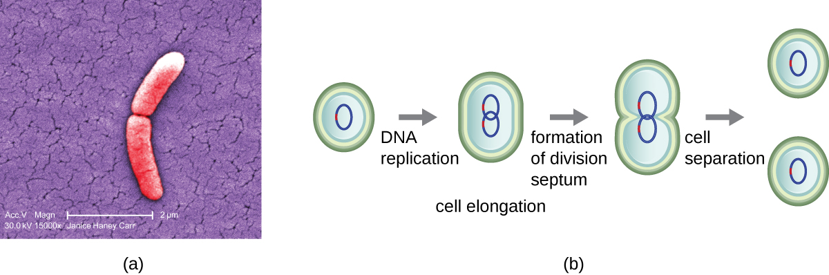
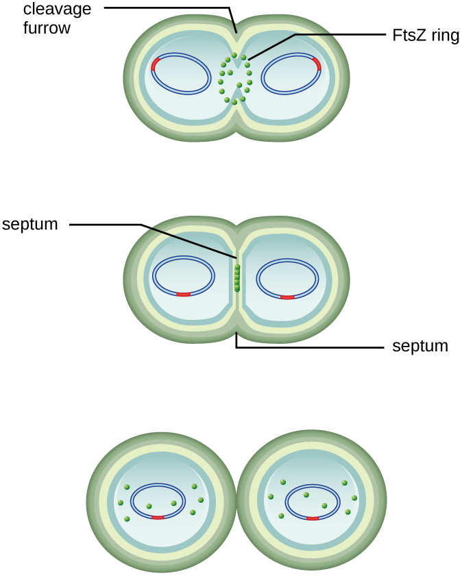
The center of the enlarged cell constricts until two daughter cells are formed, each offspring receiving a complete copy of the parental genome and a division of the cytoplasm (cytokinesis). This process of cytokinesis and cell division is directed by a protein called FtsZ. FtsZ assembles into a Z ring on the cytoplasmic membrane (Figure \(\PageIndex{2}\)). The Z ring is anchored by FtsZ-binding proteins and defines the division plane between the two daughter cells. Additional proteins required for cell division are added to the Z ring to form a structure called the divisome. The divisome activates to produce a peptidoglycan cell wall and build a septum that divides the two daughter cells. The daughter cells are separated by the division septum, where all of the cells’ outer layers (the cell wall and outer membranes, if present) must be remodeled to complete division. For example, we know that specific enzymes break bonds between the monomers in peptidoglycans and allow addition of new subunits along the division septum.

Figure \(\PageIndex{2}\): FtsZ proteins assemble to form a Z ring that is anchored to the plasma membrane. The Z ring pinches the cell envelope to separate the cytoplasm of the new cells.

Exercise \(\PageIndex{2}\)

What is the name of the protein that assembles into a Z ring to initiate cytokinesis and cell division?

Alternative Patterns of Cell Division

Binary fission is the most common pattern of cell division in prokaryotes, but it is not the only one. Other mechanisms usually involve asymmetrical division (as in budding) or production of spores in aerial filaments.

In some cyanobacteria, many nucleoids may accumulate in an enlarged round cell or along a filament, leading to the generation of many new cells at once. The new cells often split from the parent filament and float away in a process called fragmentation (Figure \(\PageIndex{15}\)). Fragmentation is commonly observed in the Actinomycetes, a group of gram-positive, anaerobic bacteria commonly found in soil. Another curious example of cell division in prokaryotes, reminiscent of live birth in animals, is exhibited by the giant bacterium Epulopiscium. Several daughter cells grow fully in the parent cell, which eventually disintegrates, releasing the new cells to the environment. Other species may form a long narrow extension at one pole in a process called budding. The tip of the extension swells and forms a smaller cell, the bud that eventually detaches from the parent cell. Budding is most common in yeast (Figure \(\PageIndex{15}\)), but it is also observed in prosthecate bacteria and some cyanobacteria.

Figure \(\PageIndex{15}\): (a) Filamentous cyanobacteria, like those pictured here, replicate by fragmentation. (b) In this electron micrograph, cells of the bacterium Gemmata obscuriglobus are budding. The larger cell is the mother cell. Labels indicate the nucleoids (N) and the still-forming nuclear envelope (NE) of the daughter cell. (credit a: modification of work by CSIRO; credit b: modification of work by Kuo-Chang Lee, Rick I Webb and John A Fuerst)

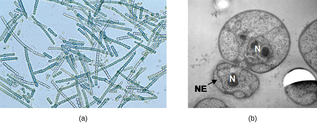
The soil bacteria Actinomyces grow in long filaments divided by septa, similar to the mycelia seen in fungi, resulting in long cells with multiple nucleoids. Environmental signals, probably related to low nutrient availability, lead to the formation of aerial filaments. Within these aerial filaments, elongated cells divide simultaneously. The new cells, which contain a single nucleoid, develop into spores that give rise to new colonies.

Generation Time

In prokaryotes (Bacteria and Archaea), the generation time, also called the doubling time, is defined as the time it takes for the population to double through one round of binary fission while dividing at a steady rate (this is in log phase; see below). Bacterial doubling times vary enormously. Whereas Escherichia coli can double in as little as 20 minutes under optimal growth conditions in the laboratory, bacteria of the same species may need several days to double in especially harsh environments. Most pathogens grow rapidly, like E. coli, but there are exceptions. For example, Mycobacterium tuberculosis, the causative agent of tuberculosis, has a generation time of between 15 and 20 hours. On the other hand, M. leprae, which causes Hansen’s disease (leprosy), grows much more slowly, with a doubling time of 14 days.

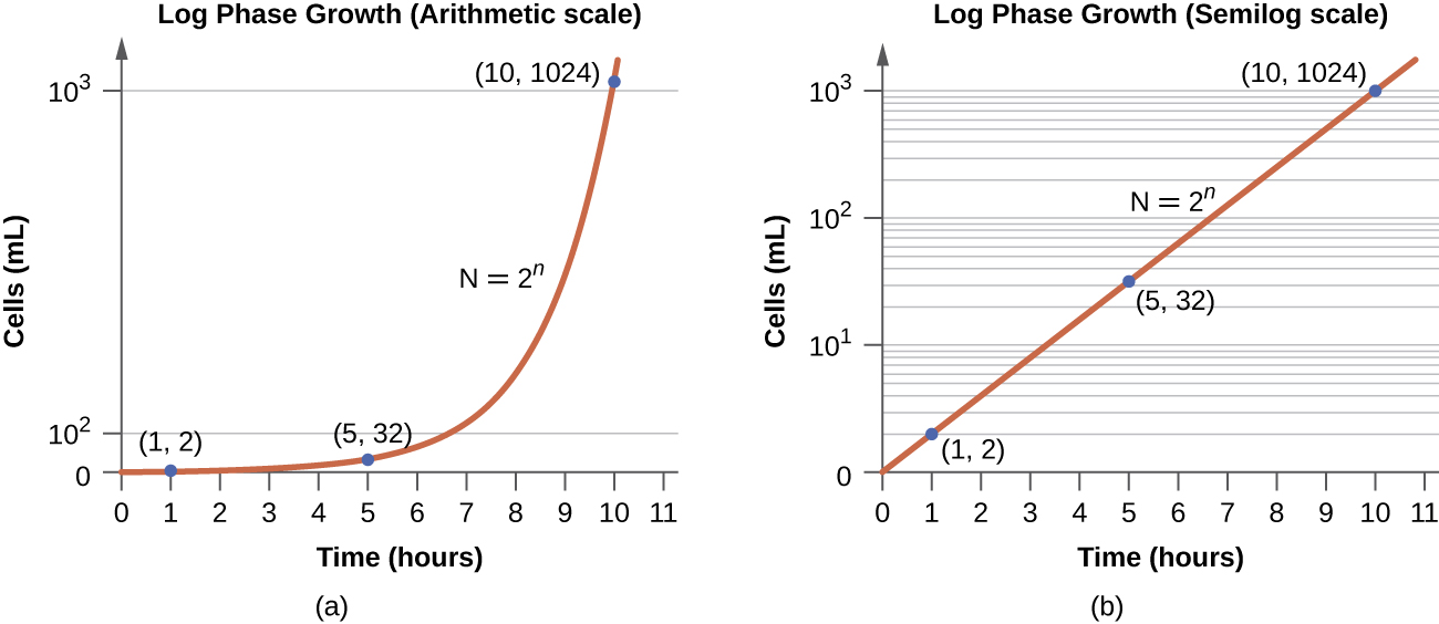
There are various mathematical methods for determining the doubling time of a microbial culture.  The most straightforward way to find the doubling time, however, is to use a growth curve such as that in Figure \(\PageIndex{5}\).  Using the growth of the culture, usually plotted on a log scale (Figure \(\PageIndex{5b}\)), the time it takes the size of the population to double during log phase can be determined.  For instance, the culture in Figure \(\PageIndex{5}\) has a population size of 1x10¹ cells/mL at a little past 3 hours.  The culture has doubled to 2x10¹ cells/mL at a little over 4 hours.  Therefore, the doubling time is approximately 1 hour (the amount of time the population took to double from 1x10¹ cells/mL to 2x10¹ cells/mL).  

Instead of doubling time, growth rate is occasionally used.  Growth rate is simply the inverse of doubling time.  Going back to the example in Figure \(\PageIndex{5}\), with a doubling time of 1 hour, the growth rate would be 1 generation per hour (because 1/1=1).  If we switch to minutes, the growth rate would be 1 generation/60 minutes which equals 0.017 generations per minute (1/60 = 0.017).

CALCULATING NUMBER OF CELLS

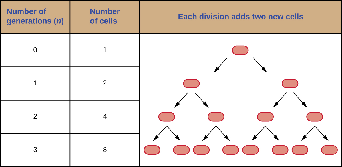
It is possible to predict the number of cells in a population when they divide by binary fission at a constant rate. As an example, consider what happens if a single cell divides every 30 minutes for 24 hours. The diagram in Figure \(\PageIndex{3}\) shows the increase in cell numbers for the first three generations.

The number of cells increases exponentially and can be expressed as 2ⁿ, where n is the number of generations. If cells divide every 30 minutes, after 24 hours, 48 divisions would have taken place. If we apply the formula 2ⁿ, where n is equal to 48, the single cell would give rise to 2⁴⁸ or 281,474,976,710,656 cells at 48 generations (24 hours). When dealing with such huge numbers, it is more practical to use scientific notation. Therefore, we express the number of cells as 2.8 × 10¹⁴ cells.

In our example, we used one cell as the initial number of cells. For any number of starting cells, the formula is adapted as follows:

\[N_n = N_02^n\]

N_n is the number of cells at any generation n, N₀ is the initial number of cells, and n is the number of generations.

Figure \(\PageIndex{3}\): The parental cell divides and gives rise to two daughter cells. Each of the daughter cells, in turn, divides, giving a total of four cells in the second generation and eight cells in the third generation. Each division doubles the number of cells.

Exercise \(\PageIndex{3}\)

With a doubling time of 30 minutes and a starting population size of 1 × 10⁵ cells, how many cells will be present after 2 hours, assuming no cell death?

The Growth Curve

Microorganisms grown in closed culture (also known as a batch culture), in which no nutrients are added and most waste is not removed, follow a reproducible growth pattern referred to as the growth curve. An example of a batch culture in nature is a pond in which a small number of cells grow in a closed environment. The culture density is defined as the number of cells per unit volume. In a closed environment, the culture density is also a measure of the number of cells in the population. Infections of the body do not always follow the growth curve, but correlations can exist depending upon the site and type of infection. When the number of live cells is plotted against time, distinct phases can be observed in the curve (Figure \(\PageIndex{4}\)).

Figure \(\PageIndex{4}\): The growth curve of a bacterial culture is represented by the logarithm of the number of live cells plotted as a function of time. The graph can be divided into four phases according to the slope, each of which matches events in the cell. The four phases are lag, log, stationary, and death.

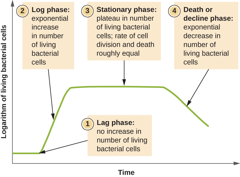
The Lag Phase

The beginning of the growth curve represents a small number of cells, referred to as an inoculum, that are added to a fresh culture medium, a nutritional broth that supports growth. The initial phase of the growth curve is called the lag phase, during which cells are gearing up for the next phase of growth. The number of cells does not change during the lag phase; however, cells grow larger and are metabolically active, synthesizing proteins needed to grow within the medium. If any cells were damaged or shocked during the transfer to the new medium, repair takes place during the lag phase. The duration of the lag phase is determined by many factors, including the species and genetic make-up of the cells, the composition of the medium, and the size of the original inoculum.

The Log Phase

In the logarithmic (log) growth phase, sometimes called exponential growth phase, the cells are actively dividing by binary fission and their number increases exponentially. For any given bacterial species, the generation time under specific growth conditions (nutrients, temperature, pH, and so forth) is genetically determined, and this generation time is called the intrinsic growth rate. During the log phase, the relationship between time and number of cells is not linear but exponential; however, the growth curve is often plotted on a semilogarithmic graph, as shown in Figure \(\PageIndex{5}\), which gives the appearance of a linear relationship.

Figure \(\PageIndex{5}\): Both graphs illustrate population growth during the log phase for a bacterial sample with an initial population of one cell and a doubling time of 1 hour. (a) When plotted on an arithmetic scale, the growth rate resembles a curve. (b) When plotted on a semilogarithmic scale (meaning the values on the y-axis are logarithmic), the growth rate appears linear.

Cells in the log phase show constant growth rate and uniform metabolic activity. For this reason, cells in the log phase are preferentially used for industrial applications and research work. This is also the phase of the growth curve used to calculated doubling time or growth rate.  The log phase is also the stage where bacteria are the most susceptible to the action of disinfectants and common antibiotics that affect protein, DNA, and cell-wall synthesis.

Stationary Phase

As the number of cells increases through the log phase, several factors contribute to a slowing of the growth rate. Waste products accumulate and nutrients are gradually used up. In addition, gradual depletion of oxygen begins to limit aerobic cell growth. This combination of unfavorable conditions slows and finally stalls population growth. The total number of live cells reaches a plateau referred to as the stationary phase (Figure \(\PageIndex{4}\)). In this phase, the number of new cells created by cell division is now equivalent to the number of cells dying; thus, the total population of living cells is relatively stagnant. The culture density in a stationary culture is constant. The culture’s carrying capacity, or maximum culture density, depends on the types of microorganisms in the culture and the specific conditions of the culture; however, carrying capacity is constant for a given organism grown under the same conditions.

During the stationary phase, cells switch to a survival mode of metabolism. As growth slows, so too does the synthesis of peptidoglycans, proteins, and nucleic-acids; thus, stationary cultures are less susceptible to antibiotics that disrupt these processes. In bacteria capable of producing endospores, many cells undergo sporulation during the stationary phase. Secondary metabolites, including antibiotics, are synthesized in the stationary phase. In certain pathogenic bacteria, the stationary phase is also associated with the expression of virulence factors, products that contribute to a microbe’s ability to survive, reproduce, and cause disease in a host organism. For example, quorum sensing in Staphylococcus aureus initiates the production of enzymes that can break down human tissue and cellular debris, clearing the way for bacteria to spread to new tissue where nutrients are more plentiful.

The Death Phase

As a culture medium accumulates toxic waste and nutrients are exhausted, cells die in greater and greater numbers. Soon, the number of dying cells exceeds the number of dividing cells, leading to an exponential decrease in the number of cells (Figure \(\PageIndex{4}\)). This is the aptly named death phase, sometimes called the decline phase. Many cells lyse and release nutrients into the medium, allowing surviving cells to maintain viability and form endospores. A few cells, the so-called persisters, are characterized by a slow metabolic rate. Persister cells are medically important because they are associated with certain chronic infections, such as tuberculosis, that do not respond to antibiotic treatment.

Sustaining Microbial Growth

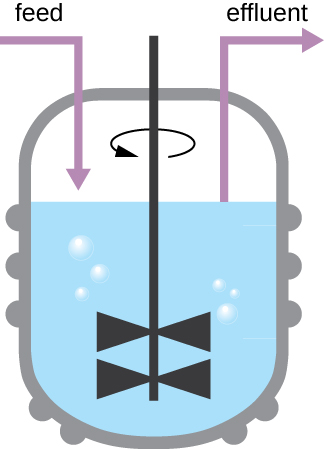
The growth pattern shown in Figure \(\PageIndex{4}\) takes place in a closed environment; nutrients are not added and waste and dead cells are not removed. In many cases, though, it is advantageous to maintain cells in the logarithmic phase of growth. One example is in industries that harvest microbial products. A chemostat (Figure \(\PageIndex{6}\)) is used to maintain a continuous culture in which nutrients are supplied at a steady rate. A controlled amount of air is mixed in for aerobic processes. Bacterial suspension is removed at the same rate as nutrients flow in to maintain an optimal growth environment.

Figure \(\PageIndex{6}\): A chemostat is a culture vessel fitted with an opening to add nutrients (feed) and an outlet to remove contents (effluent), effectively diluting toxic wastes and dead cells. The addition and removal of fluids is adjusted to maintain the culture in the logarithmic phase of growth. If aerobic bacteria are grown, suitable oxygen levels are maintained.

Exercise \(\PageIndex{4}\)

1. During which phase does growth occur at the fastest rate?
2. Name two factors that limit microbial growth.

Biofilms 

(Will be discussed in detail in Chapter 11.)

In nature, microorganisms grow mainly in biofilms, complex and dynamic ecosystems that form on a variety of environmental surfaces, from industrial conduits and water treatment pipelines to rocks in river beds. Biofilms are not restricted to solid surface substrates, however. Almost any surface in a liquid environment containing some minimal nutrients will eventually develop a biofilm. Microbial mats that float on water, for example, are biofilms that contain large populations of photosynthetic microorganisms. Biofilms found in the human mouth may contain hundreds of bacterial species. Regardless of the environment where they occur, biofilms are not random collections of microorganisms; rather, they are highly structured communities that provide a selective advantage to their constituent microorganisms.

Bacteria embedded within biofilms exhibit a higher resistance to antibiotics than their free-floating counterparts. Several hypotheses have been proposed to explain why. Cells in the deep layers of a biofilm are metabolically inactive and may be less susceptible to the action of antibiotics that disrupt metabolic activities. The polysaccharide matrix in which the cells are embedded may also slow the diffusion of antibiotics and antiseptics, preventing them from reaching cells in the deeper layers of the biofilm. Phenotypic changes may also contribute to the increased resistance exhibited by bacterial cells in biofilms. For example, the increased production of efflux pumps, membrane-embedded proteins that actively extrude antibiotics out of bacterial cells, have been shown to be an important mechanism of antibiotic resistance among biofilm-associated bacteria. Finally, biofilms provide an ideal environment for the exchange of extrachromosomal DNA, which often includes genes that confer antibiotic resistance.

Measurement of Bacterial Growth

Estimating the number of bacterial cells in a sample, known as a bacterial count, is a common task performed by microbiologists. The number of bacteria in a clinical sample serves as an indication of the extent of an infection. Quality control of drinking water, food, medication, and even cosmetics relies on estimates of bacterial counts to detect contamination and prevent the spread of disease. Two major approaches are used to measure cell number. The direct methods involve counting cells, whereas the indirect methods depend on the measurement of cell presence or activity without actually counting individual cells. Both direct and indirect methods have advantages and disadvantages for specific applications.

Plate Count

The viable plate count, or simply plate count, is a count of viable or live cells. It is based on the principle that viable cells replicate and give rise to visible colonies when incubated under suitable conditions for the specimen. The results are usually expressed as colony-forming units per milliliter (CFU/mL) rather than cells per milliliter because more than one cell may have landed on the same spot to give rise to a single colony. Furthermore, samples of bacteria that grow in clusters or chains are difficult to disperse and a single colony may represent several cells. Some cells are described as viable but nonculturable and will not form colonies on solid media. For all these reasons, the viable plate count is considered a low estimate of the actual number of live cells. These limitations do not detract from the usefulness of the method, which provides estimates of live bacterial numbers.

Microbiologists typically count plates with 30–300 colonies. Samples with too few colonies (<30) do not give statistically reliable numbers, and overcrowded plates (>300 colonies) make it difficult to accurately count individual colonies. Also, counts in this range minimize occurrences of more than one bacterial cell forming a single colony. Thus, the calculated CFU is closer to the true number of live bacteria in the population.

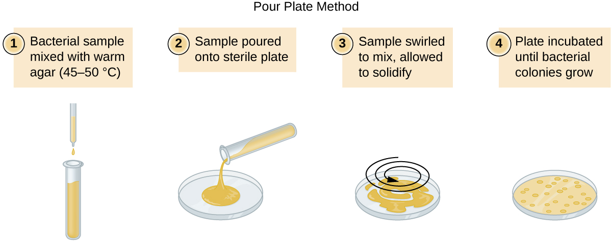
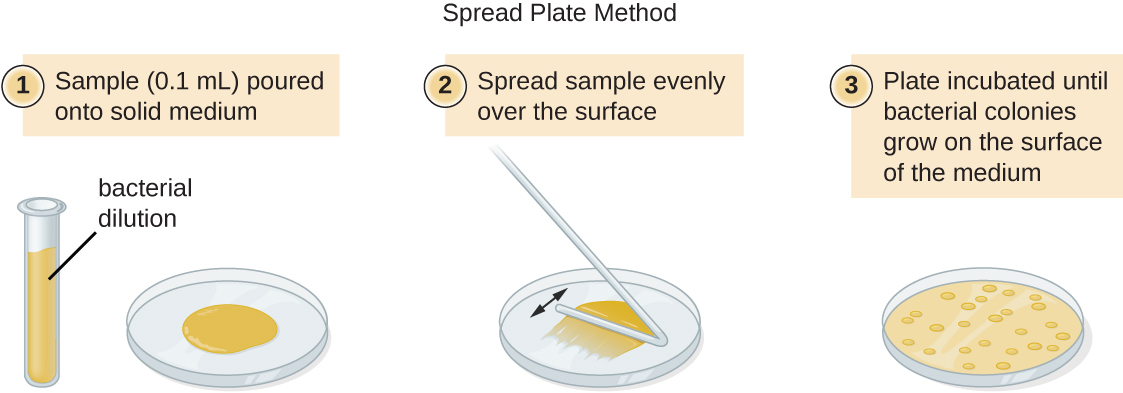
There are two common approaches to inoculating plates for viable counts: the pour plate and the spread plate methods. Although the final inoculation procedure differs between these two methods, they both start with a serial dilution of the culture.

Serial Dilution

The serial dilution of a culture is an important first step before proceeding to either the pour plate or spread plate method. The goal of the serial dilution process is to obtain plates with CFUs in the range of 30–300, and the process usually involves several dilutions in multiples of 10 to simplify calculation. The number of serial dilutions is chosen according to a preliminary estimate of the culture density. Figure \(\PageIndex{10}\) illustrates the serial dilution method.

Figure \(\PageIndex{10}\): Serial dilution involves diluting a fixed volume of cells mixed with dilution solution using the previous dilution as an inoculum. The result is dilution of the original culture by an exponentially growing factor. (credit: modification of work by “Leberechtc”/Wikimedia Commons)

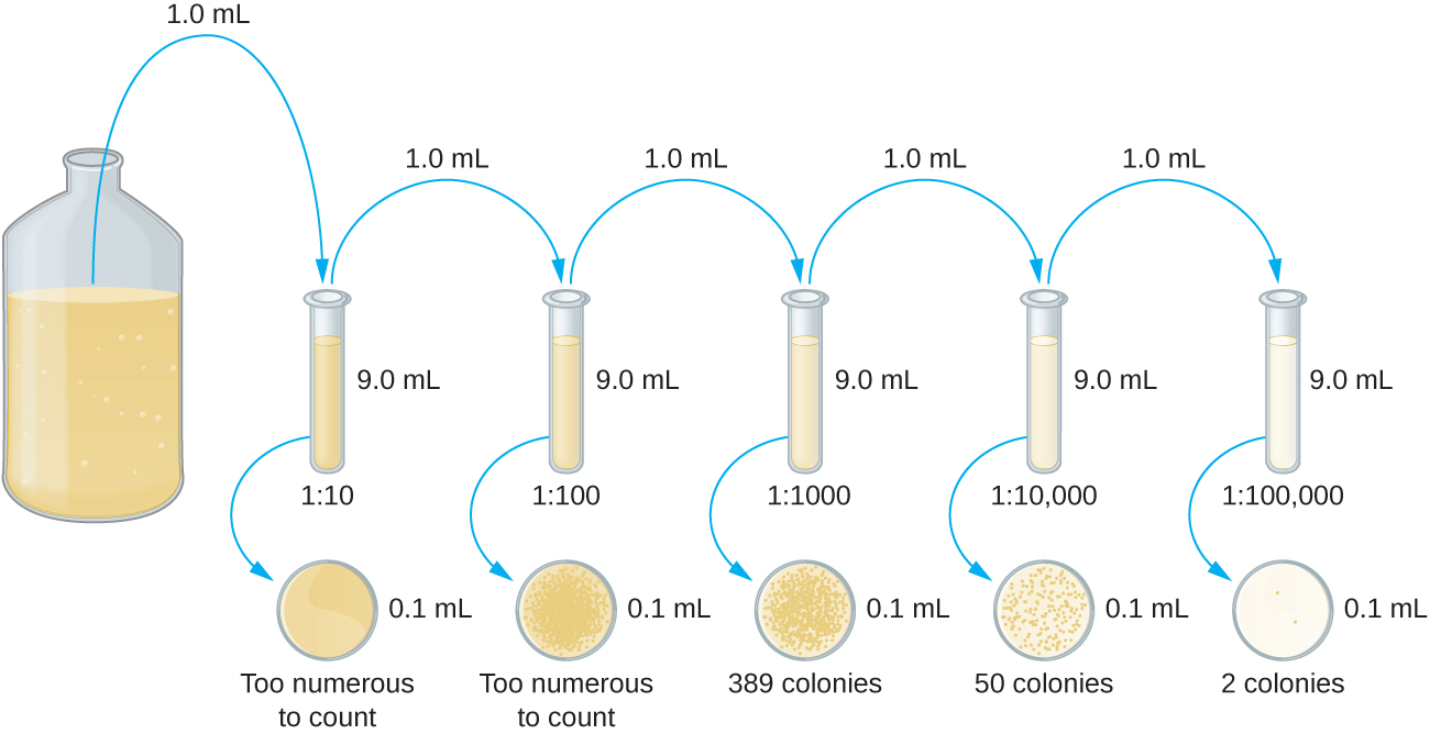
A fixed volume of the original culture, 1.0 mL, is added to and thoroughly mixed with the first dilution tube solution, which contains 9.0 mL of sterile broth. This step represents a dilution factor of 10, or 1:10, compared with the original culture. From this first dilution, the same volume, 1.0 mL, is withdrawn and mixed with a fresh tube of 9.0 mL of dilution solution. The dilution factor is now 1:100 compared with the original culture. This process continues until a series of dilutions is produced that will bracket the desired cell concentration for accurate counting. From each tube, a sample is plated on solid medium using either the pour plate method (Figure \(\PageIndex{11}\)) or the spread plate method (Figure \(\PageIndex{12}\)). The plates are incubated until colonies appear. Two to three plates are usually prepared from each dilution and the numbers of colonies counted on each plate are averaged. In all cases, thorough mixing of samples with the dilution medium (to ensure the cell distribution in the tube is random) is paramount to obtaining reliable results.

Figure \(\PageIndex{11}\): In the pour plate method of cell counting, the sample is mixed in liquid warm agar (45–50 °C) poured into a sterile Petri dish and further mixed by swirling. This process is repeated for each serial dilution prepared. The resulting colonies are counted and provide an estimate of the number of cells in the original volume sampled.

The dilution factor is used to calculate the number of cells in the original cell culture. In our example, an average of 50 colonies was counted on the plates obtained from the 1:10,000 dilution. Because only 0.1 mL of suspension was pipetted on the plate, the multiplier required to reconstitute the original concentration is 10 × 10,000. The number of CFU per mL is equal to 50 × 100 × 10,000 = 5,000,000. The number of bacteria in the culture is estimated as 5 million cells/mL. The colony count obtained from the 1:1000 dilution was 389, well below the expected 500 for a 10-fold difference in dilutions. This highlights the issue of inaccuracy when colony counts are greater than 300 and more than one bacterial cell grows into a single colony.

Figure \(\PageIndex{12}\): In the spread plate method of cell counting, the sample is poured onto solid agar and then spread using a sterile spreader. This process is repeated for each serial dilution prepared. The resulting colonies are counted and provide an estimate of the number of cells in the original volume samples.

A very dilute sample—drinking water, for example—may not contain enough organisms to use either of the plate count methods described. In such cases, the original sample must be concentrated rather than diluted before plating. This can be accomplished using a modification of the plate count technique called the membrane filtration technique. Known volumes are vacuum-filtered aseptically through a membrane with a pore size small enough to trap microorganisms. The membrane is transferred to a Petri plate containing an appropriate growth medium. Colonies are counted after incubation. Calculation of the cell density is made by dividing the cell count by the volume of filtered liquid.

Watch this video for demonstrations of serial dilutions and spread plate techniques.

 

Exercise \(\PageIndex{6}\)

1. What is a colony-forming unit?

Indirect Cell Counts

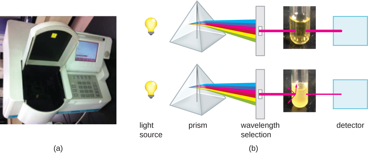
Besides direct methods of counting cells, other methods, based on an indirect detection of cell density, are commonly used to estimate and compare cell densities in a culture. The foremost approach is to measure the turbidity (cloudiness) of a sample of bacteria in a liquid suspension. The laboratory instrument used to measure turbidity is called a spectrophotometer (Figure \(\PageIndex{14}\)). In a spectrophotometer, a light beam is transmitted through a bacterial suspension, the light passing through the suspension is measured by a detector, and the amount of light passing through the sample and reaching the detector is converted to either percent transmission or a logarithmic value called absorbance (optical density). As the numbers of bacteria in a suspension increase, the turbidity also increases and causes less light to reach the detector. The decrease in light passing through the sample and reaching the detector is associated with a decrease in percent transmission and increase in absorbance measured by the spectrophotometer.

Measuring turbidity is a fast method to estimate cell density as long as there are enough cells in a sample to produce turbidity. It is possible to correlate turbidity readings to the actual number of cells by performing a viable plate count of samples taken from cultures having a range of absorbance values. Using these values, a calibration curve is generated by plotting turbidity as a function of cell density. Once the calibration curve has been produced, it can be used to estimate cell counts for all samples obtained or cultured under similar conditions and with densities within the range of values used to construct the curve.

Figure \(\PageIndex{14}\): (a) A spectrophotometer is commonly used to measure the turbidity of a bacterial cell suspension as an indirect measure of cell density. (b) A spectrophotometer works by splitting white light from a source into a spectrum. The spectrophotometer allows choice of the wavelength of light to use for the measurement. The optical density (turbidity) of the sample will depend on the wavelength, so once one wavelength is chosen, it must be used consistently. The filtered light passes through the sample (or a control with only medium) and the light intensity is measured by a detector. The light passing into a suspension of bacteria is scattered by the cells in such a way that some fraction of it never reaches the detector. This scattering happens to a far lesser degree in the control tube with only the medium. (credit a: modification of work by Hwang HS, Kim MS; credit b “test tube photos”: modification of work by Suzanne Wakim)

Measuring dry weight of a culture sample is another indirect method of evaluating culture density without directly measuring cell counts. The cell suspension used for weighing must be concentrated by filtration or centrifugation, washed, and then dried before the measurements are taken. The degree of drying must be standardized to account for residual water content. This method is especially useful for filamentous microorganisms, which are difficult to enumerate by direct or viable plate count.

Direct Cell Count

Direct cell count refers to counting the cells in a liquid culture or colonies on a plate. It is a direct way of estimating how many organisms are present in a sample. Let’s look first at a simple and fast method that requires only a specialized slide and a compound microscope.

The simplest way to count bacteria is called the direct microscopic cell count, which involves transferring a known volume of a culture to a calibrated slide and counting the cells under a light microscope. The calibrated slide is called a Petroff-Hausser chamber (Figure \(\PageIndex{7}\)) and is similar to a hemocytometer used to count red blood cells. The central area of the counting chamber is etched into squares of various sizes. A sample of the culture suspension is added to the chamber under a coverslip that is placed at a specific height from the surface of the grid. It is possible to estimate the concentration of cells in the original sample by counting individual cells in a number of squares and determining the volume of the sample observed. The area of the squares and the height at which the coverslip is positioned are specified for the chamber. The concentration must be corrected for dilution if the sample was diluted before enumeration.

Figure \(\PageIndex{7}\): (a) A Petroff-Hausser chamber is a special slide designed for counting the bacterial cells in a measured volume of a sample. A grid is etched on the slide to facilitate precision in counting. (b) This diagram illustrates the grid of a Petroff-Hausser chamber, which is made up of squares of known areas. The enlarged view shows the square within which bacteria (red cells) are counted. If the coverslip is 0.2 mm above the grid and the square has an area of 0.04 mm², then the volume is 0.008 mm³, or 0.000008 mL. Since there are 10 cells inside the square, the density of bacteria is 10 cells/0.000008 mL, which equates to 1,250,000 cells/mL. (credit a: modification of work by Jeffrey M. Vinocur)

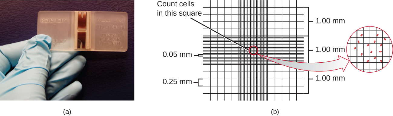
Cells in several small squares must be counted and the average taken to obtain a reliable measurement. The advantages of the chamber are that the method is easy to use, relatively fast, and inexpensive. On the downside, the counting chamber does not work well with dilute cultures because there may not be enough cells to count.

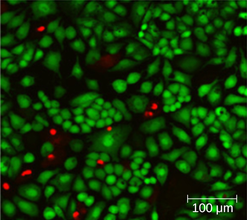
Using a counting chamber does not necessarily yield an accurate count of the number of live cells because it is not always possible to distinguish between live cells, dead cells, and debris of the same size under the microscope. However, newly developed fluorescence staining techniques make it possible to distinguish viable and dead bacteria. These viability stains (or live stains) bind to nucleic acids, but the primary and secondary stains differ in their ability to cross the cytoplasmic membrane. The primary stain, which fluoresces green, can penetrate intact cytoplasmic membranes, staining both live and dead cells. The secondary stain, which fluoresces red, can stain a cell only if the cytoplasmic membrane is considerably damaged. Thus, live cells fluoresce green because they only absorb the green stain, whereas dead cells appear red because the red stain displaces the green stain on their nucleic acids (Figure \(\PageIndex{8}\)).

Figure \(\PageIndex{8}\): Fluorescence staining can be used to differentiate between viable and dead bacterial cells in a sample for purposes of counting. Viable cells are stained green, whereas dead cells are stained red. (credit: modification of work by Panseri S, Cunha C, D’Alessandro T, Sandri M, Giavaresi G, Maracci M, Hung CT, Tampieri A)

Direct counts provide an estimate of the total number of cells in a sample. However, in many situations, it is important to know the number of live, or viable, cells. Counts of live cells are needed when assessing the extent of an infection, the effectiveness of antimicrobial compounds and medication, or contamination of food and water.

Exercise \(\PageIndex{5}\)

1. Why would you count the number of cells in more than one square in the Petroff-Hausser chamber to estimate cell numbers?
2. In the viability staining method, why do dead cells appear red?

As we have seen, methods to estimate viable cell numbers can be labor intensive and take time because cells must be grown. Recently, indirect ways of measuring live cells have been developed that are both fast and easy to implement. These methods measure cell activity by following the production of metabolic products or disappearance of reactants. Adenosine triphosphate (ATP) formation, biosynthesis of proteins and nucleic acids, and consumption of oxygen can all be monitored to estimate the number of cells.

Exercise \(\PageIndex{7}\)

1. What is the purpose of a calibration curve when estimating cell count from turbidity measurements?
2. What are the newer indirect methods of counting live cells?

 

Exercise \(\PageIndex{8}\)

Identify at least one difference between fragmentation and budding.

 

Key Concepts and Summary

• Most bacterial cells divide by binary fission. Generation time in bacterial growth is defined as the doubling time of the population.
• Other patterns of cell division include multiple nucleoid formation in cells; asymmetric division, as in budding; and the formation of hyphae and terminal spores.
• Cells in a closed system follow a pattern of growth with four phases: lag, logarithmic (exponential), stationary, and death.
• Cells can be counted by direct viable cell count. The pour plate and spread plate methods are used to plate serial dilutions into or onto, respectively, agar to allow counting of viable cells that give rise to colony-forming units. Membrane filtration is used to count live cells in dilute solutions. 
• Indirect methods can be used to estimate culture density by measuring turbidity of a culture or live cell density by measuring metabolic activity.
• Biofilms are communities of microorganisms that form when planktonic cells attach to a substrate and become sessile. Most bacteria naturally live in biofilms.
• Biofilms are commonly found on surfaces in nature and in the human body, where they may be beneficial or cause severe infections. Pathogens associated with biofilms are often more resistant to antibiotics and disinfectants.

 

Contributors and Attributions

• Nina Parker, (Shenandoah University), Mark Schneegurt (Wichita State University), Anh-Hue Thi Tu (Georgia Southwestern State University), Philip Lister (Central New Mexico Community College), and Brian M. Forster (Saint Joseph’s University) with many contributing authors. Original content via Openstax (CC BY 4.0; Access for free at https://openstax.org/books/microbiology/pages/1-introduction)