
10.2: Demographic rates
- Page ID
- 81276
\( \newcommand{\vecs}[1]{\overset { \scriptstyle \rightharpoonup} {\mathbf{#1}} } \)
\( \newcommand{\vecd}[1]{\overset{-\!-\!\rightharpoonup}{\vphantom{a}\smash {#1}}} \)
\( \newcommand{\dsum}{\displaystyle\sum\limits} \)
\( \newcommand{\dint}{\displaystyle\int\limits} \)
\( \newcommand{\dlim}{\displaystyle\lim\limits} \)
\( \newcommand{\id}{\mathrm{id}}\) \( \newcommand{\Span}{\mathrm{span}}\)
( \newcommand{\kernel}{\mathrm{null}\,}\) \( \newcommand{\range}{\mathrm{range}\,}\)
\( \newcommand{\RealPart}{\mathrm{Re}}\) \( \newcommand{\ImaginaryPart}{\mathrm{Im}}\)
\( \newcommand{\Argument}{\mathrm{Arg}}\) \( \newcommand{\norm}[1]{\| #1 \|}\)
\( \newcommand{\inner}[2]{\langle #1, #2 \rangle}\)
\( \newcommand{\Span}{\mathrm{span}}\)
\( \newcommand{\id}{\mathrm{id}}\)
\( \newcommand{\Span}{\mathrm{span}}\)
\( \newcommand{\kernel}{\mathrm{null}\,}\)
\( \newcommand{\range}{\mathrm{range}\,}\)
\( \newcommand{\RealPart}{\mathrm{Re}}\)
\( \newcommand{\ImaginaryPart}{\mathrm{Im}}\)
\( \newcommand{\Argument}{\mathrm{Arg}}\)
\( \newcommand{\norm}[1]{\| #1 \|}\)
\( \newcommand{\inner}[2]{\langle #1, #2 \rangle}\)
\( \newcommand{\Span}{\mathrm{span}}\) \( \newcommand{\AA}{\unicode[.8,0]{x212B}}\)
\( \newcommand{\vectorA}[1]{\vec{#1}} % arrow\)
\( \newcommand{\vectorAt}[1]{\vec{\text{#1}}} % arrow\)
\( \newcommand{\vectorB}[1]{\overset { \scriptstyle \rightharpoonup} {\mathbf{#1}} } \)
\( \newcommand{\vectorC}[1]{\textbf{#1}} \)
\( \newcommand{\vectorD}[1]{\overrightarrow{#1}} \)
\( \newcommand{\vectorDt}[1]{\overrightarrow{\text{#1}}} \)
\( \newcommand{\vectE}[1]{\overset{-\!-\!\rightharpoonup}{\vphantom{a}\smash{\mathbf {#1}}}} \)
\( \newcommand{\vecs}[1]{\overset { \scriptstyle \rightharpoonup} {\mathbf{#1}} } \)
\(\newcommand{\longvect}{\overrightarrow}\)
\( \newcommand{\vecd}[1]{\overset{-\!-\!\rightharpoonup}{\vphantom{a}\smash {#1}}} \)
\(\newcommand{\avec}{\mathbf a}\) \(\newcommand{\bvec}{\mathbf b}\) \(\newcommand{\cvec}{\mathbf c}\) \(\newcommand{\dvec}{\mathbf d}\) \(\newcommand{\dtil}{\widetilde{\mathbf d}}\) \(\newcommand{\evec}{\mathbf e}\) \(\newcommand{\fvec}{\mathbf f}\) \(\newcommand{\nvec}{\mathbf n}\) \(\newcommand{\pvec}{\mathbf p}\) \(\newcommand{\qvec}{\mathbf q}\) \(\newcommand{\svec}{\mathbf s}\) \(\newcommand{\tvec}{\mathbf t}\) \(\newcommand{\uvec}{\mathbf u}\) \(\newcommand{\vvec}{\mathbf v}\) \(\newcommand{\wvec}{\mathbf w}\) \(\newcommand{\xvec}{\mathbf x}\) \(\newcommand{\yvec}{\mathbf y}\) \(\newcommand{\zvec}{\mathbf z}\) \(\newcommand{\rvec}{\mathbf r}\) \(\newcommand{\mvec}{\mathbf m}\) \(\newcommand{\zerovec}{\mathbf 0}\) \(\newcommand{\onevec}{\mathbf 1}\) \(\newcommand{\real}{\mathbb R}\) \(\newcommand{\twovec}[2]{\left[\begin{array}{r}#1 \\ #2 \end{array}\right]}\) \(\newcommand{\ctwovec}[2]{\left[\begin{array}{c}#1 \\ #2 \end{array}\right]}\) \(\newcommand{\threevec}[3]{\left[\begin{array}{r}#1 \\ #2 \\ #3 \end{array}\right]}\) \(\newcommand{\cthreevec}[3]{\left[\begin{array}{c}#1 \\ #2 \\ #3 \end{array}\right]}\) \(\newcommand{\fourvec}[4]{\left[\begin{array}{r}#1 \\ #2 \\ #3 \\ #4 \end{array}\right]}\) \(\newcommand{\cfourvec}[4]{\left[\begin{array}{c}#1 \\ #2 \\ #3 \\ #4 \end{array}\right]}\) \(\newcommand{\fivevec}[5]{\left[\begin{array}{r}#1 \\ #2 \\ #3 \\ #4 \\ #5 \\ \end{array}\right]}\) \(\newcommand{\cfivevec}[5]{\left[\begin{array}{c}#1 \\ #2 \\ #3 \\ #4 \\ #5 \\ \end{array}\right]}\) \(\newcommand{\mattwo}[4]{\left[\begin{array}{rr}#1 \amp #2 \\ #3 \amp #4 \\ \end{array}\right]}\) \(\newcommand{\laspan}[1]{\text{Span}\{#1\}}\) \(\newcommand{\bcal}{\cal B}\) \(\newcommand{\ccal}{\cal C}\) \(\newcommand{\scal}{\cal S}\) \(\newcommand{\wcal}{\cal W}\) \(\newcommand{\ecal}{\cal E}\) \(\newcommand{\coords}[2]{\left\{#1\right\}_{#2}}\) \(\newcommand{\gray}[1]{\color{gray}{#1}}\) \(\newcommand{\lgray}[1]{\color{lightgray}{#1}}\) \(\newcommand{\rank}{\operatorname{rank}}\) \(\newcommand{\row}{\text{Row}}\) \(\newcommand{\col}{\text{Col}}\) \(\renewcommand{\row}{\text{Row}}\) \(\newcommand{\nul}{\text{Nul}}\) \(\newcommand{\var}{\text{Var}}\) \(\newcommand{\corr}{\text{corr}}\) \(\newcommand{\len}[1]{\left|#1\right|}\) \(\newcommand{\bbar}{\overline{\bvec}}\) \(\newcommand{\bhat}{\widehat{\bvec}}\) \(\newcommand{\bperp}{\bvec^\perp}\) \(\newcommand{\xhat}{\widehat{\xvec}}\) \(\newcommand{\vhat}{\widehat{\vvec}}\) \(\newcommand{\uhat}{\widehat{\uvec}}\) \(\newcommand{\what}{\widehat{\wvec}}\) \(\newcommand{\Sighat}{\widehat{\Sigma}}\) \(\newcommand{\lt}{<}\) \(\newcommand{\gt}{>}\) \(\newcommand{\amp}{&}\) \(\definecolor{fillinmathshade}{gray}{0.9}\)Population dynamics are often described in terms of demographic rates
Population ecologists often collect data on demographic rates: birth rates and death rates (or the converse of death rate, survival rate). Sometimes ecologists call these vital rates. Formally these are called per capita rates because they refer to the frequency of an event per individual of the population, such as births per person. Another common way to calculate rates, though not in ecology, is per annum. This is the frequency of something per year. A model set up in terms of demographic rates is called a demographic model.
While reading about mathematical models, write out the equations and make sure you understand each step of the arithmetic and algebra.
The most direct way to collect this information is if you know all of the individuals in a population (N) and you can count the number of individuals that are born and which subsequently survive until they are old enough to breed. Often we call this the birth rate, but this is not totally correct. It should really be called the “birth and survival until the next census period” rate.
We’ll stick with convention and call it the birth rate and define it like this:
\[ b = \textrm{(birth rate)} = \frac{\textrm{(number of babies)}}{\textrm{(number of adults)}} \nonumber\]
or more succinctly:
\[ b = \frac{B_t}{N_t} \]
That is, the per capita birth rate \(b\) is equal to the number of births in year t (\(B_t\)) divided by the number of adults (\(N_t\)) in the population. \(b\) is a fraction, and can take on values as low as zero. \(b = 0 \) indicates that no offspring were born, or that all offspring died before they could reproduce. \(b = 2\) indicates that two offspring were born for each adult.
Once we define \(b\) as the ratio of births to total population size, we can use algebra to set up an equation for the prediction of the actual number of births:
\[B_t = b*N_t \nonumber\]
That is, the number of organisms born and entering the population at time t (\(B_t \)) is equal to the number of organisms in the population (\(N_t \)) times the number of offspring produced per organism. Stated another way, the total number born (\(B_t \)) are often expressed as a proportion (\(b_t \)) of the number alive now (\(N_t\)).
For example, at the beginning of 1996 there were 249 elephants in the Addo Elephant National Park in South Africa (Whitehouse & Hall-Martin 2000). Over the last several decades the average birth rate was 0.0693. We can therefore use our birthrate equation to predict the number of births in 1996:
\[B_{1996} = b*N_{1996} = 0.0693*249 = 17.25 \nonumber\]
Indeed, there were 17 elephants born that year.

Figure \(\PageIndex{1}\): Elephants in Addo Elephant National Park. "Elephants at the Hapoor Dam in the park" by NJR ZA is licensed by CC BY-SA 3.0.
The per capita death rate \(d\) can be similarly defined:
\[ d = \frac{D_t}{N_t} \]
and therefore if we know the death rate and the current population size we can predict the number that will die over the next time period:
\[D_t = d*N_t \nonumber\]
The mean death rate in Addo was 0.0175; 248 elephants * 0.01750 = 4.3 predicted deaths. This is slightly fewer than the 5 that actually occurred.
So far we've only been doing some minor algebraic rearrangement of these demographic rates, but seeing how this done will help us understand how to formulate demographic models for population dynamics.
Now that we're thinking in terms of rates, we can rewrite our main population dynamics equation, which was
\[N_{t+1} = N_t − D_t + B_t \nonumber\]
in terms of demographic rates, like this:
\[N_{t+1} = N_t − d*N_t +b*N_t \nonumber\]
What this means is that if we can estimate \(d\) and \(b\), we can estimate population change without having to count up the total number of deaths and births.
In Addo Elephant National Park extensive data collection allowed researchers in the 1990s to account for all births, deaths, and surviving animals. However, if they had been unable to conduct a full population survey in 1997 they could've predicted the size of the population as
\[N_{1997} = N_{1996} − d*N_{1996} +b*N_{1996} = 249 - 0.0175*249 + 0.0693*249 \nonumber\]
This yields an estimated population size in 1997 of 262; the actual population size was 261.
If we want, we can factor out the \( N_t \) from the previous equation and get an equation like this:
\[N_{t+1} = N_t+N_t*(b−d) \nonumber\]
Ecologists usually calculate survival rates, not death rates
In our equations, \(D_t\) represents the total number of organisms that died in a given year t. The number that survived is therefore \(N_t−D_t\).
When studying population change ecologists typically work in terms of survival rates, often written as \( \phi \), the Greek letter “Phi.” The survival rate can be thought of as either a frequency or a probability. If you have 100 organisms and 50 survive to the next year, the survival rate is 0.50. Similarly, if a single organism has a 50% chance of survival over the next year, the survival rate is 0.50.
The number of deaths in a population plus the number of survivors sums to the total current population size. We therefore can use our death rate \(d\) and survival rate \(\phi \) and write:
\[N_t= \phi*N_t+d*N_t \nonumber\]
Note that in this equation we only have \(N_t\), and not dealing right now with \(N_{t+1}\).
We can do some algebra and move \(d*N_t\) using subtraction to the left of the equals sign:
\[N_t−d*N_t=\phi*N_t \nonumber\]
and see that the population size \((N_t)\) minus those which died \((d*Nt)\) equals the number of survivors \((\phi*N_t)\).
The previous equations aren't very profound - we're just accounting for the fate of all of the organisms currently in the population. Functioning population models, though, often rely on many basic mathematical manipulations in order to be set up, and we're taking the time to build up our intuition about how all the various pieces of these models work.
Another useful demonstration is this: we can also start as we just did with \(N_t=\phi*N_t+d*N_t\) and divide both sides by \(N_t\):
\[ \frac{N_t}{N_t} = \frac{\phi*N_t+d*N_t}{N_t} \nonumber\]
We can distribute the \(N_t\) on the right to give us
\[ \frac{N_t}{N_t} =\frac{\phi*N_t}{N_t} + \frac{d*N_t}{N_t} \nonumber\]
\(Nt/Nt\) cancels out on the left and the right. This gives us
\[1=\phi+d \nonumber\]
and by re-arrangement
\[1-d=\phi \nonumber\]
What does \(1=\phi+d\) mean? Again, mathematically it's a simple statement: the proportion which lived and the proportion which died over a single time step must total 1. However, keeping this manipulation in mind allows us to write out a demographic equation with some very useful features.
Let's put all of these pieces together. We'll start again with our key demographic equation using rates:
\[N_{t+1}=N_t−d*N_t +b*N_t \nonumber\]
Next, to make this clearer we'll put related terms next to each other:
\[N_{t+1}=(N_t−d*N_t)+b*N_t \nonumber\]
Now factor out \(N_{t}\) from the stuff in the parentheses:
\[N_{t+1}=N_{t}*(1−d)+b*N_{t} \nonumber\]
As we just showed, \(1=\phi+d\) and so our term \((1-d)\) can be replaced like this: \(1-d=\phi\).
Therefore, we get:
\[N_{t+1}=\phi*N_t+b*N_t \nonumber\]
This means that the number of individuals in the future \((N_{t+1})\) is comprised of those that survived \((\phi*N_t)\) and their offspring \((b*N_t)\).
In Addo Elephant National Park mean mortality was 0.0175. Mean survival is therefore 1-0.0175 = 0.9825. We therefore predict population size in the future as \(N_{t+1}=0.9825*N_t+0.06927*N_t \nonumber\)
We've now distilled down our demographic equation to predict future population size using the present population size \(N_t\), survival \(\phi\) and birth rate \(b\). While it's taken a fair bit of working with the equation, we've now reached an important breakthrough: creating a population model without determining population size at all!
If we want to be fancy we can do a bit of algebra and factor out the \(N_t\) from the previous equation:
\[N_{t+1}=N_t*(\phi+b) \nonumber\]
Let's take stock of what we've done. So far we’ve gone from our initial population models that show up in most biology textbooks but isn't really used by working ecologists:
\[N_{t+1}=N_{t}+B_t−D_t+E_t−I_t \nonumber\]
and then simplified it by ignoring immigration \(I\) and emigration \(E\), or found a population where they don’t apply or can comfortably be ignored. This gives us:
\[N_{t+1}=N_{t}+B_t−D_t \nonumber\]
Tracking total B and D is really hard -- harder than even \(N_t\) -- so we’ve done some simple thinking about population processes and some algebra to get:
\[N_{t+1}=\phi*N_t+b*N_{t} \nonumber\]
where \(\phi\)and \(b\) are usually estimated from a subset of the population. If we are confident that our survival and birth rate estimates are good, we can predict population size in the future. However, we're still relying on estimates of population size \(N_t\) which are still costly. For example, estimating the population sizes of large animals that live in open habitats such as polar bears and elephants often requires using aircraft. For animals that live in forests it can be very difficult to determine population sizes except over small areas. In the case of plants, populations are often so large that population size can only be determined for small, isolated populations. Luckily, there are some mathematical tools we can use to build meaningful population models that don't require population sizes to be estimated. To set this type of model up we'll introduce a core concept in ecology: the population growth rate.
Population dynamics are frequently described using the population growth rate
Population ecologists are frequently interested in both the absolute number of organisms (e.g. \(N_t\), \(N_{t+1}\)) and also the rate of population change over time, usually referred to as the population growth rate. The Greek letter “L” called “lambda” (\( \lambda \) ) is used to represent this rate.
If you have been following a population closely over time and have complete censuses you can calculate (\( \lambda \) ) directly using the size \((N_t)\) of the population at one time point and at a previous time point \(N_{t+1}\):
\[ \frac{N_{t+1}}{N_t} = \lambda \]
\( \lambda \) is therefore the ratio between two population sizes.
In situations where population sizes have been estimated, \( \lambda \) can be calculated directly from these data and used in subsequent models. In other cases, demographic rates (e.g. \(phi\) and \(b\)) are used to calculate it.
Case study: Calculating lambda (\( \lambda \) ) for Kirtland's Warbler:
The Kirtland’s warbler has a small geographic range and is a habitat specialist. It therefore occurs in very specific habitats, so the approximate total number of individuals could be monitored relatively easily. In 2011 there were 1828 Kirkland’s warbler males, and in 2012 there were 2090. We can therefore set up our equation with \(N_t=1828\) and \(N_{t+1}=2090\). Lambda (\( \lambda \) ) is therefore
\[ \lambda =\frac{N_{t+1}}{N_{t}}=\frac{N_{2012}}{N_{2011}} = \frac{2090}{1828} = 1.14 \]
Note that \( N_{t+1}>N_{t} \), and therefore \(\lambda > 1 \).
While the warbler population grew from 2011 to 2012, the next year in 2013 only 2020 singing males were counted. Therefore
\[ \lambda = \frac{N_{t+1}}{N_{t}} = \frac{N_{2013}}{N_{2012}} = \frac{2020}{2090} = 0.967 \nonumber\]
Note that \( N_{t+1} < N_t \), and that \( \lambda <1 \).
Once we have estimates for \( \phi \), we can make predictions about future population sizes and project population dynamics into the future. For as many years as possible, we can calculate \( N_{t+1}/N_t \); this isn’t always possible because of gaps in the data, e.g. we can’t calculate \(N_{2014}/N_{2013}\) because no data was collected in 2014.

Figure \(\PageIndex{2}\): Male Kirtland's Wabler. "Kirtland" by Bjamoros is licensed under CC BY-SA 3.0.
The value of lambda summarizes population dynamics
The minimum value \( \lambda \) can take on is 0. When \( \lambda >1 \) a population grows, while if \( \lambda <1 \) a population shrinks. If \( \lambda =1 \) the population isn’t changing. \( \lambda = 0 \) means that both adult survival \(\phi\) and reproduction \(b\) are 0. If \(\lambda=0\) the population goes extinct.
Below is a plot of the population time series next to a histogram of all of the values calculated from the time series. The time series starts in the 1970s on the left when researchers began conducting counts of all singing male Kirthland's Warblers each year. For each pair of years, \(\lambda\) was calculated to make the histogram.
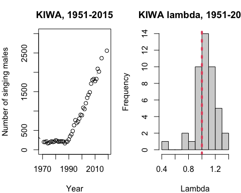
Figure \(\PageIndex{3}\): A time series (left) of the number of male Kirtland's warblers recorded and a histogram (right) of all population growth rates \((\lambda)\) calculated from the time series. The histogram shows us the distribution of observed lambda values over the ~50 year time series when KIWA males were counted every year.
What do you notice in the KIWA Lambda histogram? Why is the red line plotted and what is happening to the population at the red line?
- Answer
-
The red line 1.0 is plotted because when \(\lambda = 1\), a population is staying the same size because deaths are being balanced out by births.
Population growth rates can be calculated from demographic rates
As noted previously, it is often very difficult – if not impossible – to determine actual population sizes. For KIWA, researchers worked very hard to determine the number of males that were singing each year, but they were never completely sure if they found all of them. KIWA population is currently growing, and researchers are no longer collecting population size data, which allows allocation of research money to answer other questions, such as the expansion of the species' range into Wisconsin and Canada.
While still very challenging, it's often easier to determine demographic rates for a subset of the population, such as survival and reproduction, rather than population size. Several studies have captured KIWA males, marked them with bird bands and attempted to re-capture them each year to estimate survival rates \((\phi)\). This approach for calculating survival using mark-recapture data is similar to the one discussed in the previous chapter for calculating population size. Researchers have also found nests and determined how many baby KIWA are born per nest, and what the survival rate is for those birds until they are one year old and can breed. This gives an estimate of \(b\).
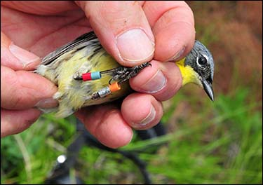
Figure \(\PageIndex{4}\): Adult Male Kirtland's Warbler being banded. Source: Source: Hanna (2015): Kirtland’s Warbler Banded as Nestling in Wisconsin Confirmed in Bahamas A Field Update. Photo by J. Trick. https://www.fws.gov/midwest/GreenBay...April2015.html
With these estimates we can calculate population growth rate \((\lambda)\) without knowing population size as:
\[ \frac{N_{t+1}}{N_t} = \phi + b \nonumber\]
We then define \(N_{t+1}/N_t\) as \(\lambda\) and so have
\[ \lambda = \phi + b \]
To show that \(\lambda\) can be defined with demographic rates as \(\lambda = \phi + b\) we start with our previous demographic equation:
\[N_{t+1}=\phi*N_t+b*N_t \nonumber\]
We can then divide both sides by Nt
\[N_{t+1}/N_t=\phi*N_t+b*N_t/N_t \nonumber\]
We can distribute the division of \(N_t\) like this
\[N_{t+1}/N_t=\phi*N_t/N_t+b*N_t/N_t \nonumber\]
This cancels out \(N_t\) entirely from the right-hand side
\[N_{t+1}/N_t= \phi + b \nonumber\]
We then define \(N_{t+1}/N_t\) as before as
\[ \lambda = \phi + b \nonumber\]
\(\lambda\) represents a combination of both survival \((\phi)\) of adults from one year to the next plus how many offspring are produced per adult and survive to reproduce themselves (b). We now have a quantity we are very interested in, the population growth rate \((\lambda)\), in terms of parameters that aren't too hard to calculate: the survival rate and birth rate ( \(\phi\) and b). This means we can understand population dynamics without needing to conduct a complete census and count every single organism -- just as long as we can track survival and reproduction on a representative subset of the population.
We could also do our math this way. We can start with
\[N_{t+1} = \phi*N_t+b*N_t \nonumber\]
and factor out \(N_t\) on the right to be:
\[N_{t+1} = N_t*(\phi + b) \nonumber\]
We then divide both sides by \(N_t\)
\[N_{t+1}/N_t=N_t+b/Nt \nonumber\]
This again gives us
\[ \frac{N_{t+1}}{N_t} = \phi +b \nonumber\]
which we write as
\[ \lambda = \phi + b \nonumber\]
Case study: Calculating Kirthland's Warbler with demographic data
We can estimate for any species if we have estimates of its adult survival rate and its birth rate. Survival for Kirtland's Warbler (KIWA) is around 67%, or 0.67. This means on average that if we have 100 adult KIWA nesting in a forest, we’d expect to see 67 of them again next year. Equivalently, we can say that an adult bird has a probability of surviving of 0.67.
The birth rate (b) is tricky to estimate for a number of reasons. Recall that b should really be called the “born and survives to reproduce” rate. Incorporating both the number of baby KIWA that hatch from eggs and their probability of surviving for one year until they can reproduce, the birth rate (b) is about 0.74.
Population growth rate is therefore
\[ \lambda = 0.67+0.74 \nonumber\]
\[ =1.3 \nonumber\]
Since \(\lambda\) >1 we’d predict that the population of KIWA will be growing. We aren’t actually counting all the birds, however.