4.2.5: Population Models

Unit 4.2.5 - Population Models

• Please read and watch the following Learning Resources
• Reading the material for understanding, and taking notes during videos, will take approximately 1 hour.
• Optional Activities are embedded.
• Bolded terms are located at the end of the unit in the Glossary. There is also a Unit Summary at the end of the Unit.
• To navigate to Unit 4.2.5, use the Contents menu at the top of the page OR the right arrow on the side of the page.
  • If on a mobile device, use the Contents menu at the top of the page OR the links at the bottom of the page.

Learning Objectives

• Compare and contrast density-dependent growth regulation and density-independent growth regulation, giving examples
• Explain the characteristics of and differences between exponential and logistic growth patterns
• Give examples of exponential and logistic growth in wild animal populations

Although life histories describe the way many characteristics of a population (such as their age structure) change over time in a general way, population ecologists make use of a variety of methods to model population dynamics mathematically. These more precise models can then be used to accurately describe changes occurring in a population and better predict future changes. Certain models that have been accepted for decades are now being modified or even abandoned due to their lack of predictive ability, and scholars strive to create effective new models.

Population Dynamics

Changes in population size over time and the processes that cause these to occur are called population dynamics. How populations change in abundance over time is a major concern of population ecology, wildlife ecology, and conservation biology, and is related to questions asked in evolutionary biology. The processes and mechanisms that drive population change are varied and include intraspecific competition with members of the same population, interspecific competition between species, the availability of food or other resources, extreme weather, inbreeding, predators or parasites.

We can consider changes in populations from various measures of populations. For example, Kirtland’s Warbler (Setophaga kirtlandii) in North America is currently:

1. Increasing in the overall number of individuals (population size).
2. Increasing in the number of occupied habitat patches (occupancy).
3. Increasing in the geographic area it occurs in (population distribution and species range).

Importantly, since the warbler prefers a certain density of Jack Pine, its density within an occupied habitat also changes. Jack Pine stands are naturally prone to burning in forest fires, and are also logged for timber. As the density of trees changes due to these disturbances, the density of warblers changes. After a fire or logging there are few if any mature pine trees and therefore few warblers. Approximately five years after seedlings have sprouted and grown up to be the proper size, the density of warblers can increase. When pine forests get too old habitat conditions are not ideal for the warbler and their abundance declines.

Population Size Over Time

Though there are many dimensions to spatial and temporal population dynamics, discussions of population dynamics often center on changes in population size over time. Changes in population size are often displayed in a time series graph with time on the x-axis (usually in years) and population size (N) on the y-axis. General patterns of population dynamics in terms of population size include:

1. Growth: Growing larger than the current size (Snail kites: Figure \(\PageIndex{1}\)a)
2. Decline: Decreasing in abundance (Elk: \(\PageIndex{1}\)b)
3. Stability: Staying approximately the same size over time (Wolves: \(\PageIndex{1}\)c)
4. Recovery: Stability or growth following a period of decline. (Impala: \(\PageIndex{1}\)d)
5. Extirpation (local extinction): Decline of one or more populations of a species to 0 (Kirtland's Warbler, \(\PageIndex{2}\)a).
6. Extinction: Decline of all members of a species to 0 (Northern White Rhino, \(\PageIndex{2}\)b).
7. Cycles: repeated patterns of growth followed by decline (Lynx: \(\PageIndex{2}\)c)

Figure \(\PageIndex{1}\): Common patterns of population change. The x-axis in all panels is the year and the y-axis is the number of individuals. a) Growth in a Florida Snail Kite (Rostrhamus sociabilis) population from 1970s to 1980s; b) Decline of the Gallatin, Montana herd of elk (Cervus canadensis) from the 1920s to 1960s; c) Stability of the Isle Royale, Michigan pack of wolves (Canis lupus) in the 1980s and 1990s; d) Recovery after population crashes in the Lake Manyara National Park, Tanzania herd of impala.

Figure \(\PageIndex{2}\): Common patterns of population change. The x-axis in all panels is the year. a) Decline to extirpation (local extinction) of Kirtland's Warbler in two populations. The y-axis is the number of singing males; b) Decline to global extinction of the Northern White Rhinoceros (Ceratotherium simum cottoni), one of two subspecies of White Rhinos. The y-axis is the total number of rhinos in the wild. c) Repeated cycling of the Canada lynx (Lynx canadensis). The y-axis is the number of lynx trapped, an index of population size.

Mixed Dynamics

Over the course of many years, a single population can display many of these dynamics. For example, Kirtland's Warbler populations were monitored by determining the number of males defending territories in their summer breeding habitat in the Great Lakes region North America, primarily Michigan. There were about 500 males with territories in the 1950s (\(\PageIndex{3}\)). The following changes occurred over the next 50 years after the species began being protected by the Endangered Species Act in the United States:

1. Decline over the course of the 1960s to ~200 territories.
2. A period of stability at ~200 territories from 1975 to 1990.
3. Steady growth to >2500 from 1990 through 2020.

Figure \(\PageIndex{3}\): Number of singing Kirtland's Warbler (Setophaga kirtlandii) males, 1950 to 2020.

Population Modeling

Researchers who study population dynamics often use mathematical models to describe and predict population dynamics and understand what factors are driving those changes. For example, if there are 2500 Kirtland’s Warblers in Michigan this year, can we predict how many will be around next year, or 10 years from now? Due to its small population size, the Kirtland’s Warbler was listed as an Endangered Species in the United States in 1967. In 2019, it was de-listed and now is considered “near-threatened.” Ecologists are very interested in using models to predict how large the Kirtland’s Warbler population will be in the future, and what factors cause it to increase and decrease. Below, we explore the conceptual and mathematical tools ecologists use to understand population dynamics and predict their future trajectories.

Types of Growth: Exponential and Logistic

Exponential Growth

Charles Darwin, in his theory of natural selection, was greatly influenced by the English clergyman Thomas Malthus. Malthus published a book in 1798 stating that populations with unlimited natural resources grow very rapidly, and then population growth decreases as resources become depleted. This accelerating pattern of increasing population size is called exponential growth.

The best example of exponential growth is seen in bacteria. Bacteria are prokaryotes that reproduce by prokaryotic fission. This division takes about an hour for many bacterial species. If 1,000 bacteria are placed in a large flask with an unlimited supply of nutrients (so the nutrients will not become depleted), after an hour, there is one round of division and each organism divides, resulting in 2,000 organisms—an increase of 1,000. In another hour, each of the 2,000 organisms will double, producing 4,000, an increase of 2,000 organisms. After the third hour, there should be 8,000 bacteria in the flask, an increase of 4,000 organisms. The important concept of exponential growth is that the population growth rate—the number of organisms added in each reproductive generation—is accelerating; that is, it is increasing at a greater and greater rate. After 1 day and 24 of these cycles, the population would have increased from 1,000 to more than 16 billion. When the population size, N, is plotted over time, a J-shaped growth curve is produced (Figure \(\PageIndex{4}\)).

Figure \(\PageIndex{4}\): When resources are unlimited, populations exhibit exponential growth, resulting in a J-shaped curve. When resources are limited, populations exhibit logistic growth. In logistic growth, population expansion decreases as resources become scarce, and it levels off when the carrying capacity of the environment is reached, resulting in an S-shaped curve.

The bacteria example is not representative of the real world where resources are limited. Furthermore, some bacteria will die during the experiment and thus not reproduce, lowering the growth rate. Therefore, when calculating the growth rate of a population, the death rate (D) (number organisms that die during a particular time interval) is subtracted from the birth rate (B) (number organisms that are born during that interval). While it is not necessary for you to know the math behind this equation, it is helpful to see how ecologists utilize math to build their models. This equation for exponentially growing population is shown here:

\[\frac{\Delta N\;(\text{change in number})} {\Delta T\;(\text{change in time})} = B\;(\text{birth rate}) - D\;(\text{death rate}) \nonumber\]

The birth rate is usually expressed on a per capita (for each individual) basis. Thus, B (birth rate) = bN (the per capita birth rate “b” multiplied by the number of individuals “N”) and D (death rate) =dN (the per capita death rate “d” multiplied by the number of individuals “N”). Additionally, ecologists are interested in the population at a particular point in time, an infinitely small time interval. For this reason, the terminology of differential calculus is used to obtain the instantaneous growth rate, replacing the change in number and time with an instant-specific measurement of number and time.

\[\frac{d N} {d T} = bN - dN = (b - d)N \nonumber\]

Notice that the “d” associated with the first term refers to the derivative (as the term is used in calculus) and is different from the death rate, also called “\(d\).” The difference between birth and death rates is further simplified by substituting the term “r” (intrinsic rate of increase) for the relationship between birth and death rates:

\[\frac{d N} {d T} = rN \nonumber\]

The value “\(r\)” can be positive, meaning the population is increasing in size; or negative, meaning the population is decreasing in size; or zero, where the population’s size is unchanging, a condition known as zero population growth. A further refinement of the formula recognizes that different species have inherent differences in their intrinsic rate of increase (often thought of as the potential for reproduction), even under ideal conditions. Obviously, a bacterium can reproduce more rapidly and have a higher intrinsic rate of growth than a human. The maximal growth rate for a species is its biotic potential, or \(r_{max}\), thus changing the equation to:

\[\frac{d N} {d T} = r_\text{max}N \nonumber\]

Video

In this 3-minute video, you will be introduced to some of the factors that limit population growth.
Question after watching: What are some of the factors that may be limiting the population growth of humans? How might they act to limit population growth?

Logistic Growth

Exponential growth is possible only when infinite natural resources are available; this is not the case in the real world. Charles Darwin recognized this fact in his description of the “struggle for existence,” which states that individuals will compete (with members of their own or other species) for limited resources. The successful ones will survive to pass on their own characteristics and traits (which we know now are transferred by DNA) to the next generation at a greater rate (natural selection). To model the reality of limited resources, population ecologists developed the logistic growth model.

Video

This 3-minute video will introduce you to the concept of carrying capacity.
Question after watching: Why are diseases considered a factor in carrying capacity?

Carrying Capacity and the Logistic Model

In the real world, with its limited resources, exponential growth cannot continue indefinitely. Exponential growth may occur in environments where there are few individuals and plentiful resources, but when the number of individuals gets large enough, resources will be depleted, slowing the growth rate. Eventually, the growth rate will plateau or level off (Figure \(\PageIndex{4}\)). This population size, which represents the maximum population size that a particular environment can support, is called the carrying capacity, or \(K\).

The formula we use to calculate logistic growth adds the carrying capacity as a moderating force in the growth rate. The expression “\(K – N\)” is indicative of how many individuals may be added to a population at a given stage, and “\(K – N\)” divided by “\(K\)” is the fraction of the carrying capacity available for further growth. Thus, the exponential growth model is restricted by this factor to generate the logistic growth equation (again, the math is not important but seeing how the model is built is):

\[\begin{align} \dfrac{d N} {d T}
&= r_\text{max} \frac{d N} {d T} \nonumber \\[5pt]
&= r_\text{max}N \frac{(K-N)} {K}\nonumber
\end{align} \nonumber\]

Notice that when \(N\) is very small, \((K-N)/K\) becomes close to \(K/K\) or \(1\), and the right side of the equation reduces to \(r_{max}N\), which means the population is growing exponentially and is not influenced by carrying capacity. On the other hand, when \(N\) is large, \((K-N)/K\) come close to zero, which means that population growth will be slowed greatly or even stopped. Thus, population growth is greatly slowed in large populations by the carrying capacity \(K\). This model also allows for the population of a negative population growth, or a population decline. This occurs when the number of individuals in the population exceeds the carrying capacity (because the value of \((K-N)/K\) is negative).

A graph of this equation yields an S-shaped curve (Figure \(\PageIndex{4}\)), and it is a more realistic model of population growth than exponential growth. There are three different sections to an S-shaped curve. Initially, growth is exponential because there are few individuals and ample resources available. Then, as resources begin to become limited, the growth rate decreases. Finally, growth levels off at the carrying capacity of the environment, with little change in population size over time.

Role of Intraspecific Competition

The logistic model assumes that every individual within a population will have equal access to resources and, thus, an equal chance for survival. For plants, the amount of water, sunlight, nutrients, and the space to grow are important resources, whereas in animals, important resources include food, water, shelter, nesting space, and mates.

In the real world, phenotypic variation among individuals within a population means that some individuals will be better adapted to their environment than others. The resulting competition between population members of the same species for resources is termed intraspecific competition (intra- = “within”; -specific = “species”). Intraspecific competition for resources may not affect populations that are well below their carrying capacity—resources are plentiful and all individuals can obtain what they need. However, as population size increases, this competition intensifies. In addition, the accumulation of waste products can reduce an environment’s carrying capacity.

Examples of Logistic Growth

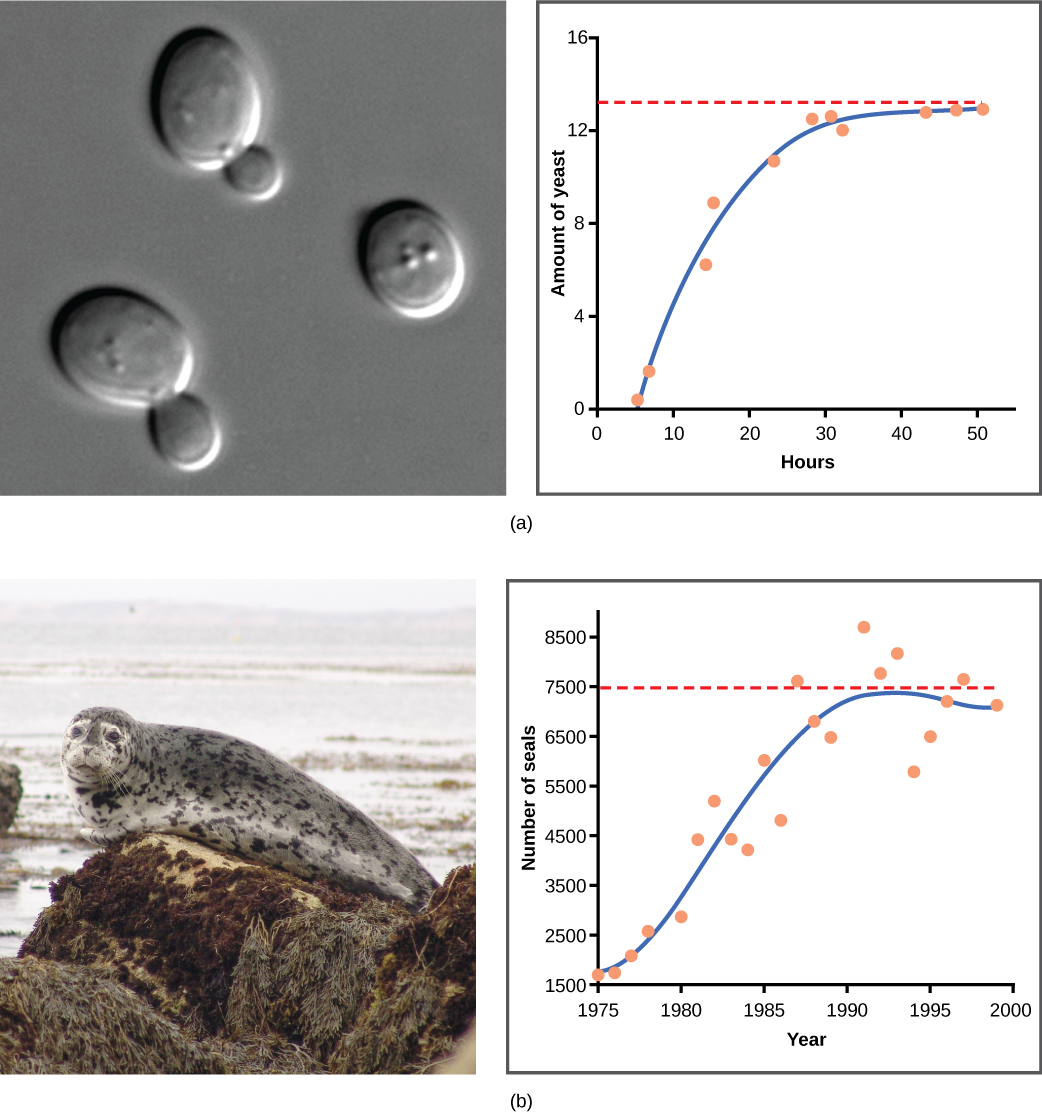
Yeast, a microscopic fungus used to make bread and alcoholic beverages, exhibits the classical S-shaped curve when grown in a test tube (Figure \(\PageIndex{5}\)a). Its growth levels off as the population depletes the nutrients that are necessary for its growth. In the real world, however, there are variations to this idealized curve. Examples in wild populations include sheep and harbor seals (Figure \(\PageIndex{5}\)b). In both examples, the population size exceeds the carrying capacity for short periods of time and then falls below the carrying capacity afterwards. This fluctuation in population size continues to occur as the population oscillates around its carrying capacity. Still, even with this oscillation, the logistic model is confirmed.

Figure \(\PageIndex{5}\): (a) Yeast grown in ideal conditions in a test tube show a classical S-shaped logistic growth curve, whereas (b) a natural population of seals shows real-world fluctuation.

Video

​

This 3-minute video reviews the various demographic models.
Question after watching: Which type of model should be applied to a perennial plant species that is introduced to a new environment without any herbivores or diseases?​

Optional Activity \(\PageIndex{1}\)

Figure \(\PageIndex{2}\)b If the major food source of the seals declines due to pollution or overfishing, which of the following would likely occur?

1. The carrying capacity of seals would decrease, as would the seal population.
2. The carrying capacity of seals would decrease, but the seal population would remain the same.
3. The number of seal deaths would increase but the number of births would also increase, so the population size would remain the same.
4. The carrying capacity of seals would remain the same, but the population of seals would decrease.

Answer

A

Optional Activity \(\PageIndex{2}\)

The maximum rate of growth of a species is called its ________.

1. limit
2. carrying capacity
3. biotic potential
4. exponential growth pattern

Answer

b. biotic potential

Population Limitations

The logistic model of population growth, while valid in many natural populations and a useful model, is a simplification of real-world population dynamics. Implicit in the model is that the carrying capacity of the environment does not change, which is not the case. The carrying capacity varies annually: for example, some summers are hot and dry whereas others are cold and wet. In many areas, the carrying capacity during winter is much lower than it is during summer. Also, natural events such as earthquakes, volcanoes, and fires can alter an environment and hence its carrying capacity. Additionally, populations do not usually exist in isolation. They engage in interspecific competition: that is, they share the environment with other species, competing with them for the same resources. These factors are also important to understanding how a specific population will grow.

Nature regulates population growth in a variety of ways. These are grouped into density-dependent factors, in which the density of the population at a given time affects growth rate and mortality, and density-independent factors, which influence mortality in a population regardless of population density. Note that in the former, the effect of the factor on the population depends on the density of the population at onset. Conservation biologists want to understand both types because this helps them manage populations and prevent extinction or overpopulation.

Video

In this 4-minute video, you will learn about density-dependent and density-independent factors that limit the growth of populations.
Question after watching: Disease is listed as a density-dependent factor limiting a population's growth. How might disease be density-dependent?

Density-Dependent Regulation

Most density-dependent factors are biological in nature (biotic) and include predation, inter- and intraspecific competition, stress, accumulation of waste, and diseases such as those caused by parasites. Usually, the denser a population is, the greater its mortality rate. For example, during intra- and interspecific competition, the reproductive rates of the individuals will usually be lower, reducing their population’s rate of growth. In addition, low prey density increases the mortality of its predator because it has more difficulty locating its food source.

An example of density-dependent regulation is shown in Figure \(\PageIndex{6}\) with results from a study focusing on the giant intestinal roundworm (Ascaris lumbricoides), a parasite of humans and other mammals. Denser populations of the parasite exhibited lower fecundity: they contained fewer eggs. One possible explanation for this is that females would be smaller in more dense populations (due to limited resources) and that smaller females would have fewer eggs. This hypothesis was tested and disproved in a 2009 study that indicated that female weight had no influence. The actual cause of the density-dependence of fecundity in this organism is still unclear and awaiting further investigation.

Figure \(\PageIndex{6}\): In this population of roundworms Ascaris lumbricoides, fecundity (number of eggs) decreases with population density (Croll et al. 1982).

Density-Independent Regulation

Many factors, typically physical or chemical in nature (abiotic), influence the mortality of a population regardless of its density, including weather, natural disasters, and pollution. An individual deer may be killed in a forest fire regardless of how many deer happen to be in that area. Its chances of survival are the same whether the population density is high or low. The same holds true for cold winter weather.

In real-life situations, population regulation is very complicated and density-dependent and independent factors can interact. A dense population that is reduced in a density-independent manner by some environmental factor(s) will be able to recover differently than a sparse population. For example, a population of deer affected by a harsh winter will recover faster if there are more deer remaining to reproduce.

Video

In this 2-minute video, you will explore biotic and abiotic limiting factors.
Question after watching: The video provides the example of a fish bowl and lists limiting factors on the growth of its fish population. Now apply this to a human population living in the "bowl" of a small town. List density-dependent, density-independent, biotic, and abiotic factors that will limit the human population's growth in that small town.

Optional Activity \(\PageIndex{3}\)

Species with limited resources usually exhibit a(n) ____ growth curve.

1. logistic
2. logical
3. experimental
4. exponential

Answer

a. logistic

Evolution Connection: Why Did the Woolly Mammoth Go Extinct?

It's easy to get lost in the discussion of dinosaurs and theories about why they went extinct 65 million years ago. Was it due to a meteor slamming into Earth near the coast of modern-day Mexico, or was it from some long-term weather cycle that is not yet understood? One hypothesis that will never be proposed is that humans had something to do with it. Mammals were small, insignificant creatures of the forest 65 million years ago, and no humans existed.

a

b

c

Figure \(\PageIndex{7}\): The three photos include: (a) 1916 mural of a mammoth herd from the American Museum of Natural History, (b) the only stuffed mammoth in the world, from the Museum of Zoology located in St. Petersburg, Russia, and (c) a one-month-old baby mammoth, named Lyuba, discovered in Siberia in 2007. (credit a: modification of work by Charles R. Knight; credit b: modification of work by “Tanapon”/Flickr; credit c: modification of work by Matt Howry)

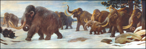
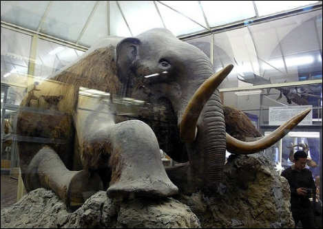
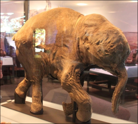
Woolly mammoths, however, began to go extinct about 10,000 years ago, when they shared the Earth with humans who were no different anatomically than humans today (Figure \(\PageIndex{7}\)). Mammoths survived in isolated island populations as recently as 1700 BC. We know a lot about these animals from carcasses found frozen in the ice of Siberia and other regions of the north like northern Canada. Scientists have sequenced at least 50 percent of its genome and believe mammoths are between 98 and 99 percent identical to modern elephants.

It is commonly thought that both climate change and human hunting led to their extinction. A 2008 study estimated that climate change reduced the mammoths' range from 8,000,000 square kilometers 42,000 years ago down to 800,000 square kilometers 6,000 years ago.⁴ It is also well documented that humans hunted these animals. A 2012 study indicated that no single factor was exclusively responsible for the extinction of these magnificent creatures.⁵ In addition to human hunting, climate change, and reduction of habitat, these scientists demonstrated another important factor in the mammoth’s extinction was the migration of humans across the Bering Strait to North America during the last ice age 20,000 years ago.

The maintenance of stable populations was and is very complex, with many interacting factors determining the outcome. It is important to remember that humans are also part of nature. We once contributed to a species’ decline using only primitive hunting technology.