10.1: Prelude - Learning the Math of Population Models

Math and mathematical models in ecology

The processes of population changes in space and time are called population dynamics. Over time, a population or species may expand its geographic range, colonize a new isolated habitat patch like an island, or disappear from areas where it occurred previously (extirpation). Even if a population or species is only found in the same locations as previously, its population size may increase or decrease, become stable, or cycle regularly.

Ecologists frequently use mathematical models to describe population dynamics. These models can be used to describe the trajectory of population growth when resources are abundant, its maximum size when resources are limited, or how rapidly in space it expands into new territory. Mathematical models can be intimidating at first, but you can start learning how they work - and how to use them yourself - with the basic tools of arithmetic and algebra most people learn in high school.

Basic mathematical models can be built using algebra

The term mathematical model perhaps sounds fancy, but in many of their forms these are just equations manipulated using standard algebra to allow us to think about how things change. In this book we'll use models for helping us think about things like populations change over time, what impact predators have on a population of its prey, and how two species using the same resource can coexist.

Here are some examples of the level of math needed to get started working with ecological models. Elsewhere we’ll investigate the applications of math in ecological modeling. Prior to studying ecology, many individuals become familiar with the equation:

\[y = M*x + B  \nonumber\]

This equation expresses a  relationship between the variables x and y. In biology, we’d call this a mathematical model and it allows us to predict x and y for particular unknowns, such as: x is the number of birds in a population this year and y is the number next year. Or, x could be the size of a plant and y is the number of seeds it produces.

A mathematical model contains both variables and parameters.  In models like ours above, x and y can be just about anything that varies between organisms or can be measured in nature: height, weight, number of species, size of a habitat, length of a river, the concentration of a toxin.  In contrast, M and B are parameters that are generally fixed for a given situation.

Solving the variable y given x

Using the above equation, if I tell you M = 1.2 and B = 10, can you calculate what y is when x = 10?  We can plug the values M = 1.2 and B = 10 into the equation:

\[ \begin{align*} y = 1.2*x \\ \end{align*} \]

We can then calculate y if x = 10.  All the values added to the equation give us this:

\[y = 1.2*10 + 10  \nonumber\]

We then do the multiplication: 

\[y = 12 + 10  \nonumber\]

The last step of addition tells us:

\[y = 22  \nonumber\]

Solving for an unknown parameter

What if I told you y = 220, x = 100, and B = 10; how would you calculate what M was? We could start like this with our known parameter (B = 10) and our values for x and y:

\[220 = M*100 + 10  \nonumber\]

We then do some algebra. First deal with the 10 by subtracting it from both sides:

\[220 - 10 = M*100 + 10 - 10  \nonumber\]

On the left, 220 - 10 = 210, and on the right 10 - 0 = 0, so this gives us:

\[210 = M*100  \nonumber\]

Now divide both sides by 100.

\[\frac{210}{100} = \frac{M*100}{100}  \nonumber\]

Which gives us:

\[\frac{210}{100} = M*1  \nonumber\]

because 100/100 = 1.

Then divide 210 by 100:

\[2.1 = M  \nonumber\]

Not too bad? The math behind basic models in ecology is often not much more involved than this. If you can work through the steps above, you can work through the population models discussed in this book.

Using mathematical models for prediction

A common use of mathematical models in ecology is prediction. For example, you can often predict the number of seeds produced by a plant using an equation like this:

\[ \textrm{(number of seeds)} = M*\textrm{(plant size)} + B  \nonumber\]

Which is the same y = M * x + B equation we just used, where y = number of seeds and x = plant size.

If M = 10, B = 15, and plant size = 30 cm tall, how many seeds would be produced?

As before we can first add the values for the parameters M and B to to model:

\[ \textrm{(number of seeds)} = 10*\textrm{(plant size)} + 15  \nonumber\]

We then plug in our particular plant size of 30 cm and do the math. First multiplication:

\[ \textrm{(number of seeds)} = 10*30 + 15 \nonumber\]

Then addition:

\[ \textrm{(number of seeds)}  = 300 + 15 \nonumber\]

\[ \textrm{(number of seeds)} = 315 \nonumber\]

So, if the equation (number of seeds) = 10 * (plant size) + 15  is accurate, a plant that is 30 cm tall would produce 315 seeds.

 

Basic population models

Population dynamics can be described with mathematical models

Populations change due to processes such as the deaths of current members of the population and the birth of new members (offspring). Discussions of population dynamics typically begin by writing out an equation which describes all of the key processes that impact population change, such as births and deaths. Most organisms live in seasonal environments, and we frequently consider changes in populations over the course of a single year, which we’ll call a one-year time step.

Let’s start building up some basic equations to describe changes in populations (population dynamics), calling the number of organisms right now N_Now and the number next year N_{Next year} (The little “Now” and “Next year” are called subscripts).

We can write out how a population change like this:

N_{Next year}=N_Now - N_{Died this year} + N_{Born this year}

When we write equations like this, we always need to remember that often represent an idealized situation; rarely can we know how large a population currently is (N_Now), and it's much harder to determine exactly how many died or were born in a given year (We’ll come back to these difficulties and their resolution in the next section on demographic models).

In addition to births and deaths, populations can also increase due to the arrival of individuals from different populations (immigration), and decrease due to the exit of current members (emigration). We therefore expand our idealized population equation to be:

N_{Next year} = N_Now - N_{Died this year} + N_{Born this year} - N_Immigrant + N_Emigrant

To make these equations more compact we often write using a more clearly expressed  notation, where a subscript of “t” = a certain time, and “t+1” equals the following time period. Often this time step is one year, but it could be any period of time relevant to the biology of an organism or is convenient to the researcher. For example, many insects grow rapidly and some go through multiple generations in a single summer, and a relevant time step could therefore be months or even weeks.

Using subscripts we can rewrite our equation as:

N_t+1 = N_t - N_{Died t} + N_{Born t} - N_{Immigrant t} + N_{Emigrant t}

where N_t+1 = N_{Next year} and N_t = N_Now.

Often in textbooks births and deaths are given their own symbols, B and D, as are immigration (I) and emigration (E). You'll therefore see this equation:

N_t+1 = N_t - D_t + B_t - I_t + E_t

or often just

N_t+1 = N_t - D + B - I + E

with subscripts only on the Ns.

 

Notation Alert!

Different authors and textbooks unfortunately use different notation, so it's important that everyone is clear what all their symbols mean, and that readers carefully determine what the symbols mean. In this case, it needs to be emphasized that N, D, B, I, and E all represent absolute numbers of individuals - they are meant to represent counts of organisms, not rates. For example, just as N_t is a count of all the individuals in the population and must be a whole number like 1000, B is a count of the number of births and must be a whole number like 5000.  In contrast, a rate would be the number of births per individual of that population.  In this case the birth rate would be B/N = 5000/1000 = 5.  Later we will use rates, like births per year, to build demographic models.

 

It is useful to remember that when you’re working with addition and subtraction you can move terms around in the equation and not alter the math. So our previous equation can be changed to this by reordering terms:

N_t+1 = N_t + B - D + E - I

Similarly, we can add parentheses to help us organize things without changing the meaning. In the equation below, the number of births (B) and deaths (D) are grouped because these are opposing processes; similarly we group E (emigration ) and I (immigration). Again, this does nothing to change the meaning.

N_t+1 = Nt + (B - D) + (E - I)

I can state the fact that these two equations are identical with an equality like this:

N_t + B - D + E - I = N_t + (B - D) + (E - I)

 

Immigration and emigration are hard to study

In the prior example, immigration and emigration were ignored. This is because immigration and emigration are very difficult to study in a population. Most populations are demographically open to immigration to some degree, especially animal populations. An open population is one that regularly receives immigrants from a nearby population. Only populations that occur on oceanic islands that are distant from the mainland or occur in other isolated chunks of habitat are likely to be closed and receive few or no immigrants.

Many habitats do have fairly rare rates of immigration, such as most islands, lakes, and isolated fragments of habitat that are surrounded by inhospitable conditions such as human structures. For example, Abuko Nature Preserve in The Gambia, West Africa is surrounded on all sides by the suburbs of the capital, Banjul.  Except for some birds, all animals found in Abuko were born there, will live their whole lives there, and never leave.   It's possible that a brave monkey may run off, but it would have to travel a considerable distance to reach the next nearest fragment of forest. For plants, most seeds will fall onto the forest floor of the preserve except those eaten by birds. These birds may happen to fly to one of the nearest forest fragments and defecate there, but it's unlikely.

Definition: Migrant

It should be noted that for human populations the general term migrant is often used to describe people moving to a different country.  In ecology, the terms migrant and migration are often reserved for species that undergo seasonal movements between habitats.

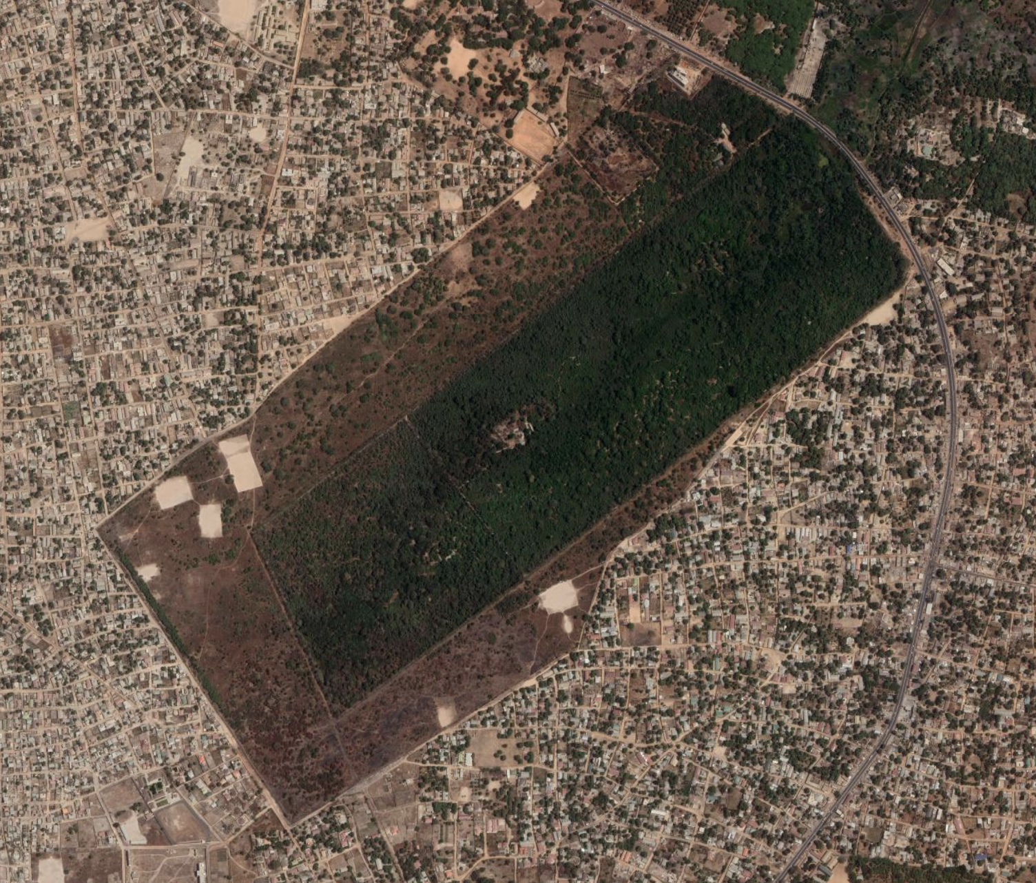
Figure \(\PageIndex{1}\): Abuko Nature Preserve, The Gambia, West Africa.  Surrounding the core forest (dark green) is more open scrub habitat (dark brown).  The preserve is entirely surrounded by residences.  Source: Google Earth: https://bit.ly/abuko00

When habitats are isolated like this, dispersal events are rare enough that they can be ignored for many ecological purposes. It should be noted, however, that while rare dispersal between populations doesn’t have much impact on population size, it can still have an impact on population genetics and evolution. Population geneticists and evolutionary biologists therefore are often interested in dispersal events that a population ecologists might ignore. A population may therefore be more or less demographically closed, but genetically open.

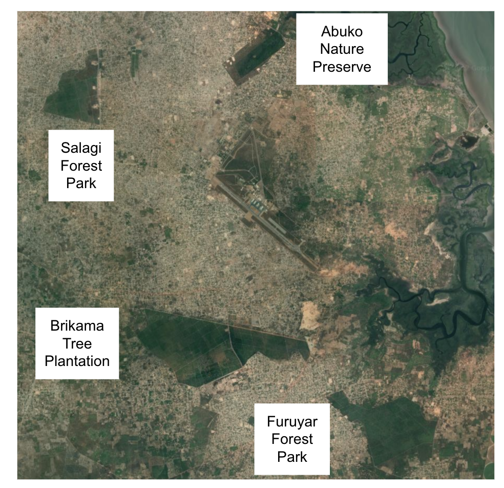
Figure \(\PageIndex{2}\): Forests nearest to Abuko Nature Preserve, The Gambia, West Africa.  Most of the terrain between the forests is either residences or agricultural land.  Source:  Google Earth: https://bit.ly/abuko1 

 

Ignoring immigration and emigration simplifies population models

Research on populations where immigration and emigration are minimal - or can justifiably be ignored - is convenient. This allows us to simplify our model of population dynamics from

N_t+1 = N_t + B - D + E - I

to one without E and I:

N_t+1 = N_t + B - D

We can therefore mathematically define a closed population as one where E = 0 and I = 0, and an open population as one where E > 0 or I > 0.

Moving forward, almost all of our population and other ecological models will ignore immigration and emigration. We will therefore be studying closed populations.  Again, few populations are truly closed!  Leaving E and I out of a model does not mean they never happen, just that they are not key players in the processes we are interested in or we are comfortable ignoring them.

While we have used a lot of symbols and equations, what we have done above presents two key creative steps in ecological modeling which are not necessarily reliant on math:

1. Brainstorming and writing out all of the key processes that can impact a population (B, D, E, I)
2. Simplifying the model by applying reasonable assumptions to make it easier to collect relevant data.

While math is important to the process, using your ecological imagination and intuition to determine what processes the equations should represent is just as important.

 

We often frame population dynamics in terms of the amount of change

Often our equation of population dynamics gets converted from focusing on the number of individuals (N_t, N_t+1) to the change in the number of individuals over time due to births and deaths.  We therefore define population change as

ΔN = B - D

Where is the Greek letter, Delta, which is used throughout science to mean "change." 

Derivation Dance

For the curious: we can arrive at the equation ΔN = B - D via some algebra by subtracting N_t from both sides of our equation.

Our equation was:

N_t+1 = N_t + B - D

We can subtract Nt from both sides:

N_t+1 - N_t = N_t + B - D - N_t

Now let’s rearrange terms for simplicity:

N_t+1 - N_t = B - D + N_t - N_t

N_t - N_t = 0, so we simplify:

N_t+1 - N_t = B - D

N_t+1 - N_t is usually written as ΔN, where is the Greek letter, Delta, which is used throughout science to mean "change". 

Looking at the equation ΔN = B - D, we can ask, “What does it mean if…”

1. B = D (B is the same as D)?
2. B > D (B is greater than D)?
3. B < D (B is less than D)?

If B = D, the number of births is balanced out by deaths and the population has not experienced a net change in size (ΔN = 0).  When B > D, births exceed deaths, ΔN is positive and the population gets bigger. When B < D, ΔN is negative and the population gets smaller.

This all may look fairly simple if math comes easily to you, but is actually kind of profound for ecological research: you can ignore how large a population actually is and still know about its population dynamics by keeping track of just births and deaths. Conversely, if you know how much a population has changed in size, you can know whether there were more births than deaths, or if deaths exceed births. As noted before, tracking individual births and deaths is hard, so gaining insights into the net number of births and deaths just from changes in population sizes is very useful. Indeed, a whole branch of population modeling is based on this (Morris and Doak 2002).