3.2.4: Life History

Life history characteristics, are those that relate to the survival, mortality, and reproduction of a species. Examples include birth rates, age at first reproduction, the number of offspring, and death rates. These characteristics evolve just like physical traits or behavior, leading to adaptations that affect population growth.

Reproductive Strategies

Population ecologists have hypothesized that suites of characteristics may evolve in species that lead to particular adaptations to their environments. These adaptations impact the kind of population growth their species experience. Population ecologists have described a continuum of life-history “strategies” with K-selected species on one end and r-selected species on the other (table \(\PageIndex{a}\)). K-selected species are adapted to stable, predictable environments. Populations of K-selected species tend to exist close to their carrying capacity (which is represented by the letter "K" in the equation for logistic population growth). These species tend to have larger, but fewer, offspring, contribute large amounts of resources to each offspring, and have long generation times. Elephants would be an example of a K-selected species (figure \(\PageIndex{a}\)). When a habitat becomes filled with a diverse collection of creatures competing with one another for the necessities of life, the advantage shifts to K-strategists. K-strategists have stable populations that are close to K. There is nothing to be gained from a high growth rate (r). The species will benefit most by a close adaptation to the conditions of its environment.

Table \(\PageIndex{a}\): Comparison of K- and r-selected species

Characteristics of K-selected species	Characteristics of r-selected species
Mature late	Mature early
Greater longevity	Lower longevity
Increased parental care	Decreased parental care
Strong competitors	Weak competitors (strong colonizers)
Fewer offspring	More offspring
Larger offspring	Smaller offspring

Figure \(\PageIndex{a}\): (a) Elephants are considered K-selected species as they live long, mature late, and provide long-term parental care to few offspring. Oak trees produce many offspring that do not receive parental care, but are considered K-selected species based on longevity and late maturation. (b) Dandelions and jellyfish are both considered r-selected species as they mature early, have short lifespans, and produce many offspring that receive no parental care.

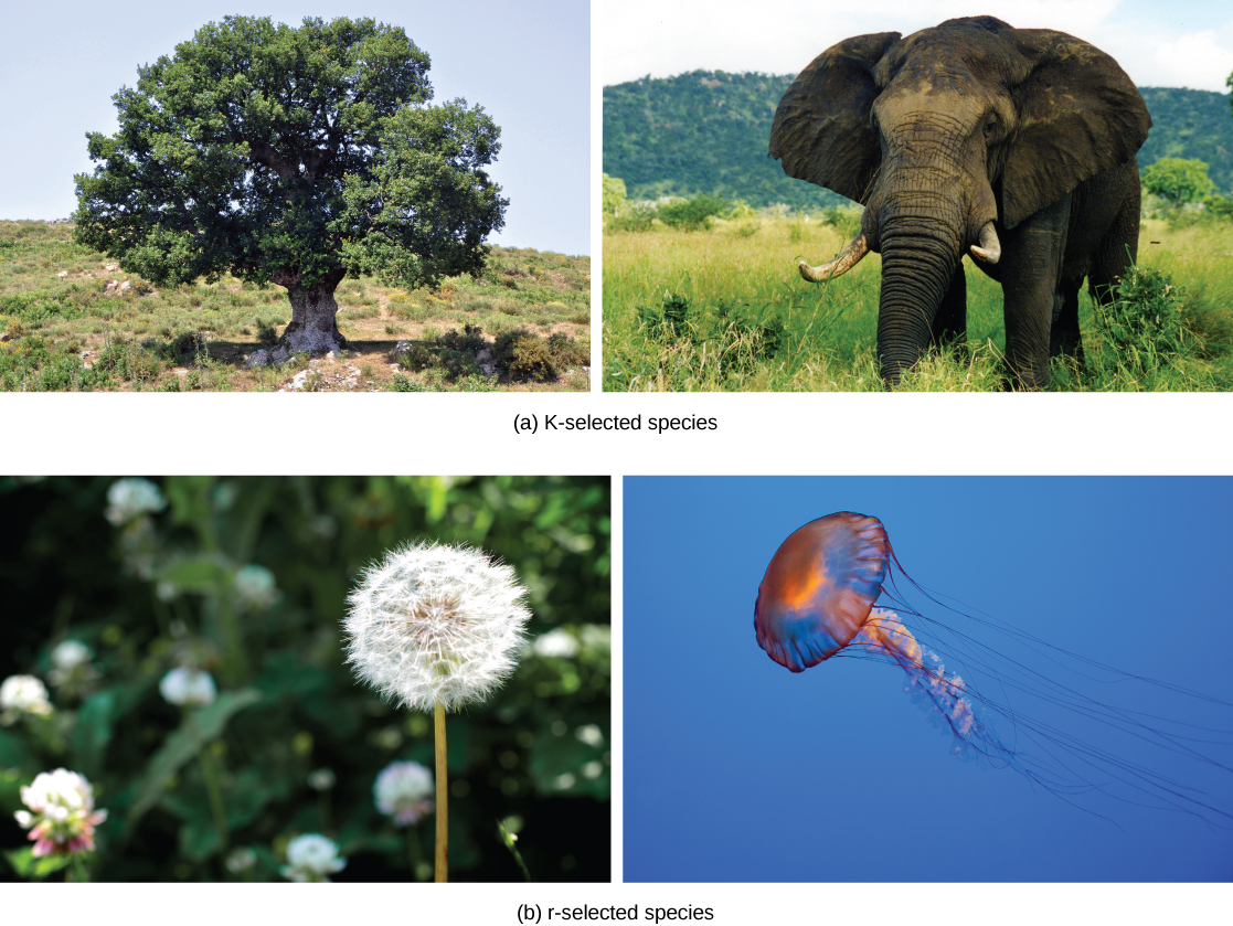
r-selected species are adapted to unstable and unpredictable environments. They have large numbers of small offspring. Animals that are r-selected do not provide a lot of resources or parental care to offspring, and the offspring are relatively self-sufficient at birth. Examples of r-selected species are marine invertebrates such as jellyfish and plants such as the dandelion (figure \(\PageIndex{a}\)). r-strategists have short life spans and reproduce quickly, resulting in short generation times. For example, the housefly can produce 7 generations each year (each of about 120 young). Ragweed is well-adapted to exploiting its environment in a hurry - before competitors can become established. It grows rapidly and produces a huge number of seeds (after releasing its pollen, the bane of many hay fever sufferers). Because ragweed's approach to continued survival is through rapid reproduction (a high value of r) it is called an r-strategist. Other weeds, many insects, and many rodents are also r-strategists. If fact, if we consider an organism a pest, it is probably an r-strategist.

The two extreme strategies are at two ends of a continuum on which real species life histories will exist. In addition, life history strategies do not need to evolve as suites but can evolve independently of each other; therefore, each species may have some characteristics that trend toward one extreme or the other. Nevertheless, the r- and K-selection theory provides a foundation for a more accurate life history framework. New demographic-based models of life history evolution have been developed, which incorporate many ecological concepts included in r- and K-selection theory as well as population age structure and mortality factors.

Life Tables

Life tables provide important information about the life history of an organism and the life expectancy of individuals at each age. They are modeled after actuarial tables used by the insurance industry for estimating human life expectancy. Life tables may include the probability of each age group dying before their next birthday, the percentage of surviving individuals dying at a particular age interval (their mortality rate, and their life expectancy at each interval). An example of a life table is shown in Table \(\PageIndex{b}\) from a study of Dall mountain sheep, a species native to northwestern North America. Notice that the population is divided into age intervals (column A).

As can be seen from the mortality rate data (column D), a high death rate occurred when the sheep were between six months and a year old, and then increased even more from 8 to 12 years old, after which there were few survivors. The data indicate that if a sheep in this population were to survive to age one, it could be expected to live another 7.7 years on average, as shown by the life-expectancy numbers in column E. Life tables often include more information than shown in Table \(\PageIndex{b}\), such as fecundity (reproduction) rates for each age group. 

Table \(\PageIndex{b}\): Life Table of Dall Mountain Sheep

Age interval (years)	Number dying in age interval out of 1000 born	Number surviving at beginning of age interval out of 1000 born	Mortality rate per 1000 alive at beginning of age interval	Life expectancy or mean lifetime remaining to those attaining age interval
0–0.5	54	1000	54.0	7.06
0.5–1	145	946	153.3	—
1–2	12	801	15.0	7.7
2–3	13	789	16.5	6.8
3–4	12	776	15.5	5.9
4–5	30	764	39.3	5.0
5–6	46	734	62.7	4.2
6–7	48	688	69.8	3.4
7–8	69	640	107.8	2.6
8–9	132	571	231.2	1.9
9–10	187	439	426.0	1.3
10–11	156	252	619.0	0.9
11–12	90	96	937.5	0.6
12–13	3	6	500.0	1.2
13–14	3	3	1000	0.7

Survivorship Curves

Another tool used by population ecologists is a survivorship curve, which is a graph of the number of individuals surviving at each age interval versus time. These curves allow us to compare the life histories of different populations (figure \(\PageIndex{c}\)). There are three types of survivorship curves. In a type I survivorship curve, mortality is low in the early and middle years and occurs mostly in older individuals. Organisms exhibiting a type I survivorship typically produce few offspring and provide good care to the offspring increasing the likelihood of their survival. Humans and most mammals exhibit a type I survivorship curve. In type II survivorship curves, mortality is relatively constant throughout the entire life span, and mortality is equally likely to occur at any point in the life span. Many bird populations provide examples of an intermediate or type II survivorship curve. In type III survivorship curves, early ages experience the highest mortality with much lower mortality rates for organisms that make it to advanced years. Type III organisms typically produce large numbers of offspring, but provide very little or no care for them. Trees and marine invertebrates exhibit a type III survivorship curve because very few of these organisms survive their younger years, but those that do make it to an old age are more likely to survive for a relatively long period of time.

Figure \(\PageIndex{c}\): Survivorship curves show the chance of survival in a population according to age. The number of individuals surviving (on a log scale) is on the y-axis, and time (representing relative age) is on the x-axis. Humans and most mammals have a Type I survivorship curve, because death primarily occurs in the older years. The Type I survivorship curve is represented by a convex curve, which rapidly declines at the end. Birds have a Type II survivorship curve, as death at any age is equally probable. The Type II survivorship curve is represented by a straight line, going from the upper left to lower right of the graph. Trees have a Type III survivorship curve because very few survive the younger years, but after a certain age, individuals are much more likely to survive. The Type III survivorship curve is represented by a concave curve, which initially declines rapidly and then flattens.

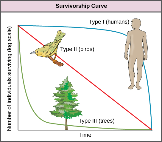
While is no exact association between reproductive strategies (K- or r-selected) and survivorship curves (Type I, II, or III), K-selected species are more likely to have a Type III survivorship curve. r-selected species tend to have a Type I survivorship curve.

Attribution

Modified by Melissa Ha from the following sources:

• Population Dynamics and Regulation from General Biology by OpenStax (CC-BY)
• Population Demographics and Dynamics from Environmental Biology by Matthew R. Fisher (CC-BY)
• Principles of Population Growth from Biology by John W. Kimball (CC-BY)