3.2.3: Population Growth and Regulation

Population ecologists make use of a variety of methods to model population dynamics. An accurate model should be able to describe the changes occurring in a population and predict future changes. The two simplest models of population growth use deterministic equations (equations that do not account for random events) to describe the rate of change in the size of a population over time. The first of these models, exponential growth, describes populations that increase in numbers without any limits to their growth. The second model, logistic growth, introduces limits to reproductive growth that become more intense as the population size increases. Neither model adequately describes natural populations, but they provide points of comparison.

The Population Growth Rate (r )

The population growth rate (sometimes called the rate of increase or per capita growth rate, r) equals the birth rate (b) minus the death rate (d) divided by the initial population size (N₀).

Another method of calculating the population growth rate involves final and initial population size (figure \(\PageIndex{a}\)). In this case, population growth rate (r) equals the final population size (N) minus the initial population size (N₀) and divided by the initial population size (N₀).

Figure \(\PageIndex{a}\): How could we calculate the growth rate of this caribou population per year if there were 200 individuals in 2016 and 300 individuals in 2018? Image by K. Joly/NPS (public domain).

Doubling Time

The doubling time is how long it will take for a population to become twice its initial size. The doubling time (t) is equal to 0.69 divided by the population growth rate (r), written as a proportion.

Population ecologists sometimes round this equation and calculate doubling time using the "Rule of 70" (dividing 70 by the population growth rate, written as a percentage). To express population growth rate as a percentage, it is multiplied by 100%. Thus, the 0.69 in the original doubling time equation is also multiplied by 100. This value (69) is rounded to 70 for simplicity.

Exponential Growth

Charles Darwin, in developing his theory of natural selection, was influenced by the English clergyman Thomas Malthus. Malthus published his book in 1798 stating that populations with abundant natural resources grow very rapidly. However, they limit further growth by depleting their resources. The early pattern of accelerating population size is called exponential growth (figure \(\PageIndex{b}\)).

Figure \(\PageIndex{b}\): These graphs show exponential and logistic growth, with population size on the y-axis and time on the x-axis. When resources are unlimited, populations exhibit (a) exponential growth, shown in a J-shaped curve. When resources are limited, populations exhibit (b) logistic growth. In logistic growth, population expansion decreases as resources become scarce, and it levels off when the carrying capacity of the environment is reached. The logistic growth curve is S-shaped.

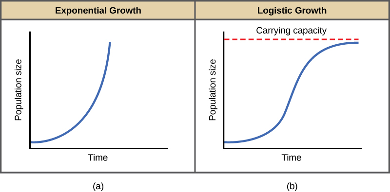
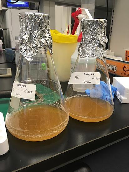
The best example of exponential growth in organisms is seen in bacteria. Bacteria are prokaryotes that reproduce quickly, about an hour for many species. If 1000 bacteria are placed in a large flask with an abundant supply of nutrients (so the nutrients will not become quickly depleted), the number of bacteria will have doubled from 1000 to 2000 after just an hour (figure \(\PageIndex{c}\)). In another hour, each of the 2000 bacteria will divide, producing 4000 bacteria. After the third hour, there should be 8000 bacteria in the flask. The important concept of exponential growth is that the growth rate—the number of organisms added in each reproductive generation—is itself increasing; that is, the population size is increasing at a greater and greater rate. After 24 of these cycles, the population would have increased from 1000 to more than 16 billion bacteria. When the population size, N, is plotted over time, a J-shaped growth curve is produced (figure \(\PageIndex{b}\)).

Figure \(\PageIndex{c}\): Bacteria growing with abundant nutrients in a flask will exhibit exponential growth. Image by Soledad Mirand-Rottman (CC-BY-SA).

The bacteria-in-a-flask example is not truly representative of the real world where resources are usually limited. However, when a species is introduced into a new habitat that it finds suitable, it may show exponential growth for a while. In the case of the bacteria in the flask, some bacteria will die during the experiment and thus not reproduce; therefore, the growth rate is lowered from a maximal rate in which there is no mortality.

Logistic Growth

Extended exponential growth is possible only when infinite natural resources are available; this is not the case in the real world. Charles Darwin recognized this fact in his description of the “struggle for existence,” which states that individuals will compete, with members of their own or other species, for limited resources. The successful ones are more likely to survive and pass on the traits that made them successful to the next generation at a greater rate (natural selection). To model the reality of limited resources, population ecologists developed the logistic growth model.

In the real world, with its limited resources, exponential growth cannot continue indefinitely. Exponential growth may occur in environments where there are few individuals and plentiful resources, but when the number of individuals gets large enough, resources will be depleted and the growth rate will slow down. Eventually, the growth rate will plateau or level off (figure \(\PageIndex{b}\)). This population size, which is determined by the maximum population size that a particular environment can sustain, is called the carrying capacity, symbolized as K. In real populations, a growing population often overshoots its carrying capacity and the death rate increases beyond the birth rate causing the population size to decline back to the carrying capacity or below it. Most populations usually fluctuate around the carrying capacity in an undulating fashion rather than existing right at it.

A graph of logistic growth yields the S-shaped curve (figure \(\PageIndex{b}\)). It is a more realistic model of population growth than exponential growth. There are three different sections to an S-shaped curve. Initially, growth is exponential because there are few individuals and ample resources available. Then, as resources begin to become limited, the growth rate decreases. Finally, the growth rate levels off at the carrying capacity of the environment, with little change in population number over time.

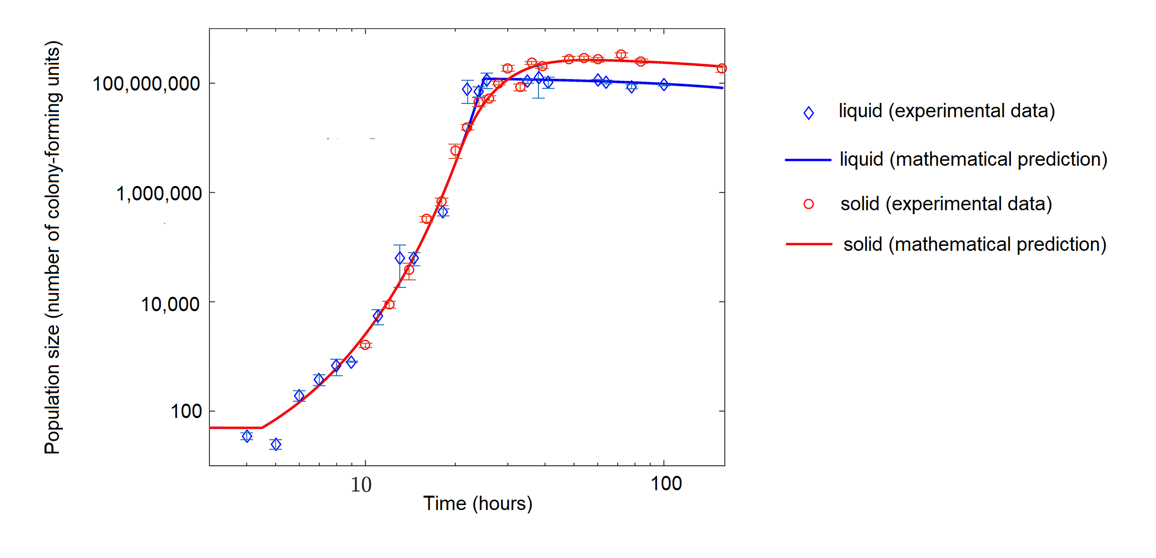
While bacteria in a flask with abundant nutrients might initially exhibit exponential growth, bacteria grown with limited nutrients can exhibit logistic growth (figure \(\PageIndex{d}\)). 

Figure \(\PageIndex{d}\): The growth of the bacterium Escherichia coli (E. coli) with limited nutrients over time in hours. Population size is in number of colony-forming units, which is a cell capable of dividing to produce a colony of cells. The bacteria were grown in liquid (blue diamonds) or on a semisolid medium (agar, red circles). The points represent actual measurements of populations size, and the lines represent a mathematical model, basically a prediction that is based on the data points. The data show logistic population growth, particularly in solid media. Initially, population size increases rapidly (concave part of curve), but the growth rate then stabilizes (straight line) before decreasing (convex part of curve) and leveling near the carrying capacity. Image modified from Shao X, Mugler A, Kim J, Jeong HJ, Levin BR, Nemenman I (2017) Growth of bacteria in 3-d colonies. PLoS Comput Biol 13(7): e1005679 (CC-BY).

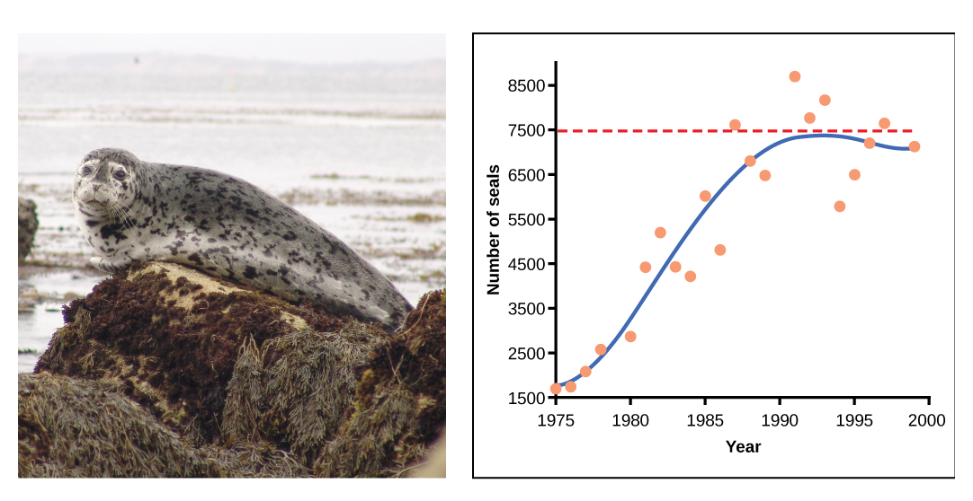
In some populations, there are variations to the S-shaped curve. Examples in wild populations include sheep and harbor seals (figure \(\PageIndex{e}\)). In both examples, the population size exceeds the carrying capacity for short periods of time and then falls below the carrying capacity afterwards. This fluctuation in population size continues to occur as the population oscillates around its carrying capacity. Still, even with this oscillation the logistic model is confirmed.

Figure \(\PageIndex{e}\): A natural population of seals shows logistic growth. The number of seals, ranging from 1500 to 8500, is on the y-axis, and the year, ranging from 1975-2000, is on the x-axis. Orange dots represent the observed population size each year, and the blue line represent the trend. From 1975 to 1983, the blue line curves upwards, representing an increase in both population size and population growth rate. From 1983 to 1992, the curve flattens, representing that population size is still increasing, but population growth rate is decreasing. After 1992, population fluctuates near the carrying capacity (dotted, horizontal line). 

The logistic population growth model is not the only way that populations respond to limited resources. In some populations, growth is exponential until resources run low, wastes accumulate, or disease spreads (see limiting factors below), and the population then crashes. Thus, population growth rate (and size) may plummet rapidly instead of tapering as it approaches the carrying capacity. 

Population Dynamics and Regulation

The logistic model of population growth, while valid in many natural populations and a useful model, is a simplification of real-world population dynamics. Implicit in the model is that the carrying capacity of the environment does not change, which is not the case. The carrying capacity varies annually. For example, some summers are hot and dry whereas others are cold and wet; in many areas, the carrying capacity during the winter is much lower than it is during the summer. Furthermore, some factors (growth factors) increase population growth rate while other factors (limiting factors) slow population growth. Examples of growth factors are resources like food, water, and space. Limiting factors can be classified as density-dependent or density-independent.

Density-dependent Regulation

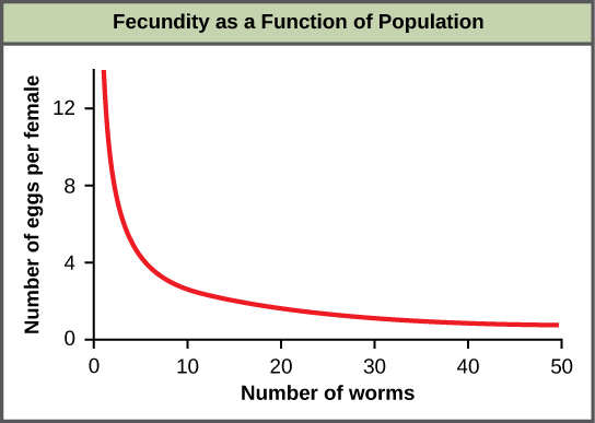
Most density-dependent factors are biological in nature (biotic). Usually, the denser a population is, the greater its mortality rate. An example of density-dependent regulation is shown in figure \(\PageIndex{f}\) with results from a study focusing on the giant intestinal roundworm (Ascaris lumbricoides), a parasite of humans and other mammals. Denser populations of the parasite exhibited lower fecundity: they contained fewer eggs. One possible explanation for this is that females would be smaller in more dense populations (due to limited resources) and that smaller females would have fewer eggs. This hypothesis was tested and disproved in a 2009 study which showed that female weight had no influence. The actual cause of the density-dependence of fecundity in this organism is still unclear and awaiting further investigation.

Figure \(\PageIndex{f}\): In this population of roundworms, fecundity (number of eggs per female) decreases with population size (number of worms). (Note that population size rather than population density is shown here, but population density does correlate with population size.) The number of eggs decreases rapidly at first, then levels off between 30 to 50 worms.

Density-dependent factors include predation, parasitism, herbivory, competition, and accumulation of waste. As a population increases, its predators are able to harvest it more easily. Prey density also affects population growth rate of predators: low prey density increases the mortality of its predator because it has more difficulty locating its food sources.

Parasites are able to pass from host to host more easily as the population density of the host increases. For this reason, epidemics among humans are particularly severe in cities. In fact, for most of the period since humans began living in cities, city populations have been maintained only through continual immigration from the countryside. Not until the development of community sanitation, immunization, and other public health measures did cities avoid periodic sharp drops in population as a result of epidemics. The recurrent epidemics of the "black death" in Europe that began in the fourteenth century caused a sharp decline in population. In just three years (1348–1350), at least one-quarter of the population of Europe died from the disease (probably plague). 

Similarly, herbivores can more easily spread between individual plants in a dense population. This is why strip cropping (see Sustainable Agriculture) helps control pests. An herbivore or plant pathogen may infect one row of plants, but it is less likely to spread to more distant rows of that species.

While interspecific competition occurs between different species, intraspecific competition occurs when members of the same species harm each other by using the same resources. For example, in the summer of 1980, much of southern New England was struck by an infestation of the gypsy moth (figure \(\PageIndex{g}\)). As the summer wore on, the larvae (caterpillars) pupated, the hatched adults mated, the females laid masses of eggs (each mass containing several hundred eggs) on virtually every tree in the region. In early May of 1981, the young caterpillars that hatched from these eggs began feeding and molting.

Figure \(\PageIndex{g}\): Gypsy moth caterpillars face intraspecific competition at high densities. Image by Editor at Large (CC-BY-SA).

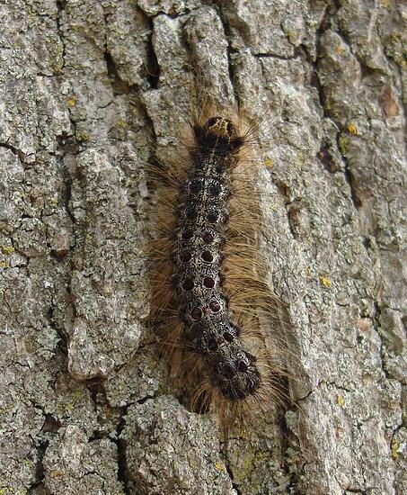
The results were dramatic: In 72 hours, a 50-ft beech tree or a 25-ft white pine tree would be completely defoliated. Large patches of forest began to take on a winter appearance with their skeletons of bare branches. In fact, the infestation was so heavy that many trees were completely defoliated before the caterpillars could complete their larval development. The result: a massive die-off of the animals; very few succeeded in completing metamorphosis. Here, then, was a dramatic example of how competition among members of one species for a finite resource - in this case, food - caused a sharp drop in population. The effect was clearly density-dependent. The lower population densities of the previous summer had permitted most of the animals to complete their life cycle. 

Density-independent Regulation

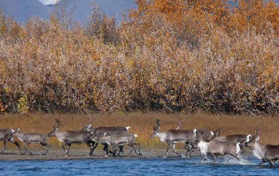
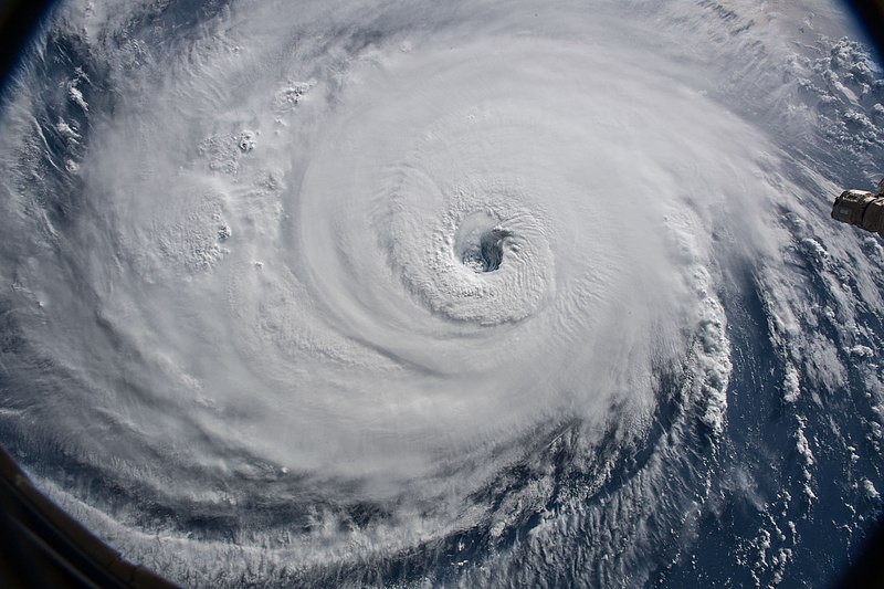
Density-independent factors, typically physical or chemical in nature (abiotic), influence the mortality of a population regardless of its density, including weather (figure \(\PageIndex{h}\)), natural disasters (earthquakes, volcanoes, fires, etc.), and pollution. An individual deer may be killed in a forest fire regardless of how many deer happen to be in that area. Its chances of survival are the same whether the population density is high or low. The same holds true for cold winter weather.

Figure \(\PageIndex{h}\): Severe weather, like Hurricane Florence of 2018, can reduce population size regardless of density. Image by NASA Goddard Space Flight Center (CC-BY)

In real-life situations, population regulation is very complicated and density-dependent and independent factors can interact. A dense population that is reduced in a density-independent manner by some environmental factor(s) will be able to recover differently than a sparse population. For example, a population of deer affected by a harsh winter will recover faster if there are more deer remaining to reproduce.

Attributions

Modified by Melissa Ha from the following sources:

• Population Growth and Regulation from Environmental Biology by Matthew R. Fisher (CC-BY)
• Principles of Population Growth and The Human Population from Biology by John W. Kimball (CC-BY)
• Population Dynamics and Regulation from General Biology by OpenStax (CC-BY)