
2.5: The Needleman-Wunsch Algorithm


- Last updated
- Mar 17, 2021
- Save as PDF

( \newcommand{\kernel}{\mathrm{null}\,}\)
We will now use dynamic programming to tackle the harder problem of general sequence alignment. Given two strings S=(S1,...,Sn) and T=(T1,...,Tm), we want to find the longest common subsequence, which may or may not contain gaps. Rather than maximizing the length of a common subsequence we want to compute the common subsequence that optimizes the score as defined by our scoring function. Let d denote the gap penalty cost and s(x;y) the score of aligning a base x and a base y. These are inferred from insertion/deletion and substitution probabilities which can be determined experimentally or by looking at sequences that we know are closely related. The algorithm we will develop in the following sections to solve sequence alignment is known as the Needleman-Wunsch algorithm.
Dynamic programming vs. memoization
Before we dive into the algorithm, a final note on memoization is in order. Much like the Fibonacci problem, the sequence alignment problem can be solved in either a top-down or bottom-up approach.
In a top-down recursive approach we can use memoization to create a potentially large dictionary indexed by each of the subproblems that we are solving (aligned sequences). This requires O(n2m2) space if we index each subproblem by the starting and end points of the subsequences for which an optimal alignment needs to be computed. The advantage is that we solve each subproblem at most once: if it is not in the dictionary, the problem gets computed and then inserted into dictionary for further reference.
In a bottom-up iterative approach we can use dynamic programming. We define the order of computing sub-problems in such a way that a solution to a problem is computed once the relevant sub-problems have been solved. In particular, simpler sub-problems will come before more complex ones. This removes the need for keeping track of which sub-problems have been solved (the dictionary in memoization turns into a matrix) and ensures that there is no duplicated work (each sub-alignment is computed only once).
Thus in this particular case, the only practical difference between memoization and dynamic programming is the cost of recursive calls incurred in the memoization case (space usage is the same).
Problem Statement
Suppose we have an optimal alignment for two sequences S1…n and T1…m in which Si matches Tj. The key insight is that this optimal alignment is composed of an optimal alignment between (S1,…,Si−1) and (T1,…,Ti−1) and an optimal alignment between (Si+1,…,Sn) and (Tj+1,…,Tm). This follows from a cut-and-paste argument: if one of these partial alignments is suboptimal, then we cut-and-paste a better alignment in place of the suboptimal one. This achieves a higher score of the overall alignment and thus contradicts the optimality of the initial global alignment. In other words, every subpath in an optimal path must also be optimal. Notice that the scores are additive, so the score of the overall alignment equals the addition of the scores of the alignments of the subsequences. This implicitly assumes that the sub-problems of computing the optimal scoring alignments of the subsequences are independent. We need to biologically motivate that such an assumption leads to meaningful results.
Index space of subproblems
We now need to index the space of subproblems. Let Fi,j be the score of the optimal alignment of (S1,…,Si) and (T1,…,Ti). The space of subproblems is {Fi,j,i∈[0,|S|],j∈[0,|T|]}. This allows us to maintain an (m+1)×(n+1) matrix F with the solutions (i.e. optimal scores) for all the subproblems.
Local optimality
We can compute the optimal solution for a subproblem by making a locally optimal choice based on the results from the smaller sub-problems. Thus, we need to establish a recursive function that shows how the solution to a given problem depends on its subproblems. And we use this recursive definition to fill up the table F in a bottom-up fashion.
We can consider the 4 possibilities (insert, delete, substitute, match) and evaluate each of them based on the results we have computed for smaller subproblems. To initialize the table, we set F0,j=−j·d and Fi,0=−i·d since those are the scores of aligning (T1,…,Ti) with j gaps and (S1,…,Si) with i gaps (aka zero overlap between the two sequences). Then we traverse the matrix column by column computing the optimal score for each alignment subproblem by considering the four possibilities:
• Sequence S has a gap at the current alignment position.
• Sequence T has a gap at the current alignment position.
• There is a mutation (nucleotide substitution) at the current position.
• There is a match at the current position.
We then use the possibility that produces the maximum score. We express this mathematically by the recursive formula for Fi,j:
F(0,0)=0
Initialization:F(i,0)=F(i−1,0)−d
F(0,j)=F(0,j−1)−d
Iteration:F(i,j)=max{F(i−1,j)−d insert gap in SF(i,j−1)−d insert gap in TF(i−1,j−1)+s(xi,yj) match or mutation
Termination : Bottom right
After traversing the matrix, the optimal score for the global alignment is given by Fm,n. The traversal order needs to be such that we have solutions to given subproblems when we need them. Namely, to compute Fi,j, we need to know the values to the left, up, and diagonally above Fi,j in the table. Thus we can traverse the table in row or column major order or even diagonally from the top left cell to the bottom right cell. Now, to obtain the actual alignment we just have to remember the choices that we made at each step.
Optimal Solution
Paths through the matrix F correspond to optimal sequence alignments. In evaluating each cell Fi,j we make a choice by selecting the maximum of the three possibilities. Thus the value of each (uninitialized) cell in the matrix is determined either by the cell to its left, above it, or diagonally to the left above it. A match and a substitution are both represented as traveling in the diagonal direction; however, a different cost can be applied for each, depending on whether the two base pairs we are aligning match or not. To construct the actual optimal alignment, we need to traceback through our choices in the matrix. It is helpful to maintain a pointer for each cell while filling up the table that shows which choice was made to get the score for that cell. Then we can just follow our pointers backwards to reconstruct the optimal alignment.
Solution Analysis
The runtime analysis of this algorithm is very simple. Each update takes O(1) time, and since there are mn elements in the matrix F, the total running time is O(mn). Similarly, the total storage space is O(mn). For the more general case where the update rule is more complicated, the running time may be more expensive. For instance, if the update rule requires testing all sizes of gaps (e.g. the cost of a gap is not linear), then the running time would be O(mn(m+n)).
Needleman-Wunsch in practice
Assume we want to align two sequences S and T, where
S = AGT
T = AAGC
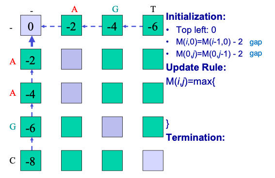
The first step is placing the two sequences along the margins of a matrix and initializing the matrix cells. To initialize we assign a 0 to the first entry in the matrix and then fill in the first row and column based on the incremental addition of gap penalties, as in Figure 2.9 below. Although the algorithm could fill in the first row and column through iteration, it is important to clearly define and set boundaries on the problem.
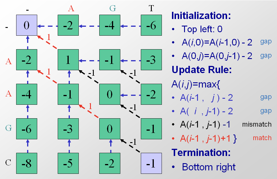
The next step is iteration through the matrix. The algorithm proceeds either along rows or along columns, considering one cell at time. For each cell three scores are calculated, depending on the scores of three adjacent matrix cells (specifically the entry above, the one diagonally up and to the left, and the one to the left). The maximum score of these three possible tracebacks is assigned to the entry and the corresponding pointer is also stored. Termination occurs when the algorithm reaches the bottom right corner. In Figure 2.10 the alignment matrix for sequences S and T has been filled in with scores and pointers.
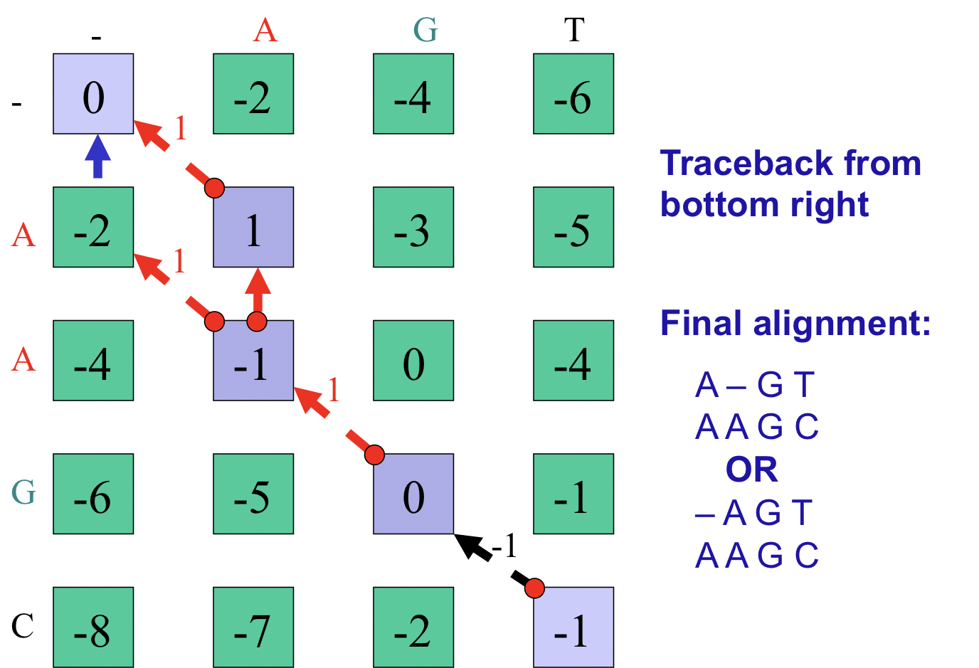
The final step of the algorithm is optimal path traceback. In our example we start at the bottom right corner and follow the available pointers to the top left corner. By recording the alignment decisions made at each cell during traceback, we can reconstruct the optimal sequence alignment from end to beginning and then invert it. Note that in this particular case, multiple optimal pathways exist (Figure 2.11). A pseudocode implementation of the Needleman-Wunsch algorithm is included in Appendix 2.11.4
Optimizations
The dynamic algorithm we presented is much faster than the brute-force strategy of enumerating alignments and it performs well for sequences up to 10 kilo-bases long. Nevertheless, at the scale of whole genome alignments the algorithm given is not feasible. In order to align much larger sequences we can make modifications to the algorithm and further improve its performance.
Bounded Dynamic Programming
One possible optimization is to ignore Mildly Boring Alignments (MBAs), or alignments that have too many gaps. Explicitly, we can limit ourselves to stay within some distance W from the diagonal in the matrix
F of subproblems. That is, we assume that the optimizing path in F from F0,0 to Fm,n is within distance W along the diagonal. This means that recursion (2.2) only needs to be applied to the entries in F within distance W around the diagonal, and this yields a time/space cost of O((m+n)W) (refer to Figure 2.12).
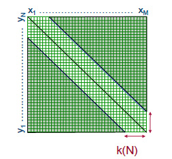
Figure 2.12: Bounded dynamic programming example
Note, however, that this strategy is heuristic and no longer guarantees an optimal alignment. Instead it attains a lower bound on the optimal score. This can be used in a subsequent step where we discard the recursions in matrix F which, given the lower bound, cannot lead to an optimal alignment.
Linear Space Alignment
Recursion (2.2) can be solved using only linear space: we update the columns in F from left to right during which we only keep track of the last updated column which costs O(m) space. However, besides the score Fm,n of the optimal alignment, we also want to compute a corresponding alignment. If we use trace back, then we need to store pointers for each of the entries in F, and this costs O(mn) space.
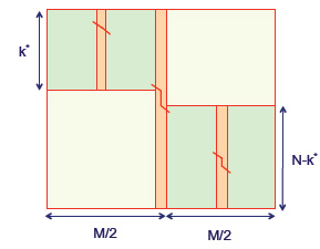
Figure 2.13: Recovering the sequence alignment with O(m+n) space
It is also possible to find an optimal alignment using only linear space! The goal is to use divide and conquer in order to compute the structure of the optimal alignment for one matrix entry in each step. Figure 2.13 illustrates the process. The key idea is that a dynamic programming alignment can proceed just as easily in the reverse direction, starting at the bottom right corner and terminating at the top left. So if the matrix is divided in half, then both a forward pass and a reverse pass can run at the same time and converge in the middle column. At the crossing point we can add the two alignment scores together; the cell in the middle column with the maximum score must fall in the overall optimal path.
We can describe this process more formally and quantitatively. First compute the row index u∈1,...,m that is on the optimal path while crossing the n2th column. For 1≤i≤m and n≤j≤n let Ci,j denote the row index that is on the optimal path to Fi,j while crossing then2th column. Then, while we update the columns of F from left to right, we can also update the columns of C from left to right. So, in O(mn) time and O(m)space we are able to compute the score Fm,n and also Cm,n, which is equal to the row index u∈1,...,m that is on the optimal path while crossing the n2th column. Now the idea of divide and conquer kicks in. We repeat the above procedure for the upper left u×n2 submatrix of F and also repeat the above procedure for the lower right (m−u)×n2 submatrix of F . This can be done using O(m+n) allocated linear space. The running time for the upper left submatrix is O(un2) and the running time for the lower right submatrix is O((m−u)n2), which added together gives a running time of O(mn2)=O(mn).
We keep on repeating the above procedure for smaller and smaller submatrices of F while we gather more and more entries of an alignment with optimal score. The total running time is O(mn)+O(mn2)+O(mn4)+…=O(2mn)=O(mn). So, without sacrificing the overall running time (up to a constant factor), divide and conquer leads to a linear space solution (see also Section ?? on Lecture 3).