2.2: Aligning Sequences

Sequence alignment represents the method of comparing two or more genetic strands, such as DNA or RNA. These comparisons help with the discovery of genetic commonalities and with the (implicit) tracing of strand evolution. There are two main types of alignment:

• Global alignment: an attempt to align every element in a genetic strand, most useful when the genetic strands under consideration are of roughly equal size. Global alignment can also end in gaps.
• Local alignment: an attempt to align regions of sequences that contain similar sequence motifs within a larger context.

Example Alignment

Within orthologous gene sequences, there are islands of conservation, or relatively large stretches of nucleotides that are preserved between generations. These conserved regions typically imply functional elements and vice versa. As an example, we considered the alignment of the Gal10-Gal1 intergenic region for four different yeast species, the first cross-species whole genome alignment (Figure 2.1). As we look at this alignment, we note that some areas are more similar than others, suggesting that these areas have been conserved through evolution. In particular, we note some small conserved motifs such as CGG and CGC, which in fact are functional elements in the binding of Gal4[8].² This example highlights how evolutionary data can help locate functional areas of the genome: per-nucleotide levels of conservation denote the importance of each nucleotide, and exons are among the most conserved elements in the genome.

We have to be cautious with our interpretations, however, because conservation does sometimes occur by random chance. In order to extract accurate biological information from sequence alignments we have to separate true signatures from noise. The most common approach to this problem involves modeling the evolutionary process. By using known codon substitution frequencies and RNA secondary structure constraints, for example, we can calculate the probability that evolution acted to preserve a biological function. See Chapter ?? for an in-depth discussion of evolutionary modeling and functional conservation in the context of genome annotation.

Solving Sequence Alignment

Genomes change over time, and the scarcity of ancient genomes makes it virtually impossible to compare the genomes of living species with those of their ancestors. Thus, we are limited to comparing just the genomes of living descendants. The goal of sequence alignment is to infer the ‘edit operations’ that change a genome by looking only at these endpoints.

We must make some assumptions when performing sequence alignment, if only because we must transform a biological problem into a computationally feasible one and we require a model with relative simplicity and tractability. In practice, sequence evolution is mostly due to nucleotide mutations, deletions, and insertions (Figure 2.2). Thus, our sequence alignment model will only consider these three operations and will ignore other realistic events that occur with lower probability (e.g. duplications).³

1. A nucleotide mutation occurs when some nucleotide in a sequence changes to some other nucleotide during the course of evolution.
2. A nucleotide deletion occurs when some nucleotide is deleted from a sequence during the course of evolution.

   

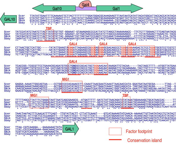
   © source unknown. All rights reserved. This content is excluded from our Creative Commons license. For more information, see http://ocw.mit.edu/help/faq-fair-use/.

   Figure 2.1: Sequence alignment of Gal10-Gal1 between four yeast strains. Asterisks mark conserved nucleotides.

3. A nucleotide insertion occurs when some nucleotide is added to a sequence during the course of evolution.

Figure 2.2: Evolutionary changes of a genetic sequence

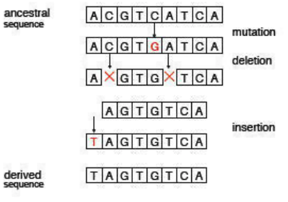
Note that these three events are all reversible. For example, if a nucleotide N mutates into some nucleotide M, it is also possible that nucleotide M can mutate into nucleotide N. Similarly, if nucleotide N is deleted, the event may be reversed if nucleotide N is (re)inserted. Clearly, an insertion event is reversed by a corresponding deletion event.

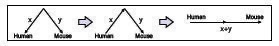
This reversibility is part of a larger design assumption: time-reversibility. Specifically, any event in our model is reversible in time. For example, a nucleotide deletion going forward in time may be viewed as a nucleotide insertion going backward in time. This is useful because we will be aligning sequences which both exist in the present. In order to compare evolutionary relatedness, we will think of ourselves following one sequence backwards in time to a common ancestor and then continuing forward in time to the other sequence. In doing so, we can avoid the problem of not having an ancestral nucleotide sequence.

Note that time-reversibility is useful in solving some biological problems but does not actually apply to

Figure 2.3: Aligning human to mouse sequences is analogous to tracing backward from the human to a common ancestor, then forward to the mouse

biological systems. For example, CpG4^₄ may incorrectly pair with a TpG or CpA during DNA replication, but the reverse operation cannot occur; hence this transformation is not time-reversible. To be very clear, time-reversibility is simply a design decision in our model; it is not inherent to the biology⁵.

We also need some way to evaluate our alignments. There are many possible sequences of events that could change one genome into another. Perhaps the most obvious ones minimize the number of events (i.e., mutations, insertions, and deletions) between two genomes, but sequences of events in which many insertions are followed by corresponding deletions are also possible. We wish to establish an optimality criterion that allows us to pick the ‘best’ series of events describing changes between genomes.

We choose to invoke Occam’s razor and select a maximum parsimony method as our optimality criterion. That is, in general, we wish to minimize the number of events used to explain the differences between two nucleotide sequences. In practice, we find that point mutations are more likely to occur than insertions and deletions, and certain mutations are more likely than others[11]. Our parsimony method must take these and other inequalities into account when maximizing parsimony. This leads to the idea of a substitution matrix and a gap penalty, which are developed in the following sections. Note that we did not need to choose a maximum parsimony method for our optimality criterion. We could choose a probabilistic method, for example using Hidden Markov Models (HMMs), that would assign a probability measure over the space of possible event paths and use other methods for evaluating alignments (e.g., Bayesian methods). Note the duality between these two approaches: our maximum parsimony method reflects a belief that mutation events have low probability, thus in searching for solutions that minimize the number of events we are implicitly maximizing their likelihood.

---

2. Gal4 in fact displays a particular structure, comprising two arms that each bind to the same sequence, in reversed order.

3. Interestingly, modeling decisions taken to improve tractability do not necessarily result in diminished relevance; for example, accounting for directionality in the study of chromosome inversions yields polynomial-time solutions to an otherwise NP problem.[6]

4. p denotes the phosphate backbone in a DNA strand

5. This is an example where understanding the biology helps the design greatly, and illustrates the general principle that success in computational biology requires strong knowledge of the foundations of both CS and biology. Warning: computer scientists who ignore biology will work too hard.