2.4: Dynamic Programming

Before proceeding to a solution of the sequence alignment problem, we first discuss dynamic programming, a general and powerful method for solving problems with certain types of structure.

Theory of Dynamic Programming

Dynamic programming may be used to solve problems with:

1. Optimal Substructure: The optimal solution to an instance of the problem contains optimal solutions to subproblems.
2. Overlapping Subproblems: There are a limited number of subproblems, many/most of which are repeated many times.

Dynamic programming is usually, but not always, used to solve optimization problems, similar to greedy algorithms. Unlike greedy algorithms, which require a greedy choice property to be valid, dynamic programming works on a range of problems in which locally optimal choices do not produce globally optimal results. Appendix 2.11.3 discusses the distinction between greedy algorithms and dynamic programming in more detail; generally speaking, greedy algorithms solve a smaller class of problems than dynamic programming.

In practice, solving a problem using dynamic programming involves two main parts: Setting up dynamic programming and then performing computation. Setting up dynamic programming usually requires the following 5 steps:

1. Find a ’matrix’ parameterization of the problem. Determine the number of dimensions (variables).
2. Ensure the subproblem space is polynomial (not exponential). Note that if a small portion of subproblems are used, then memoization may be better; similarly, if subproblem reuse is not extensive, dynamic programming may not be the best solution for the problem.
3. Determine an effective transversal order. Subproblems must be ready (solved) when they are needed, so computation order matters.

4. Determine a recursive formula: A larger problem is typically solved as a function of its subparts.

5. Remember choices: Typically, the recursive formula involves a minimization or maximization step. More- over, a representation for storing transversal pointers is often needed, and the representation should be polynomial.

Once dynamic programming is setup, computation is typically straight-forward:
1. Systematically fill in the table of results (and usually traceback pointers) and find an optimal score.

2. Traceback from the optimal score through the pointers to determine an optimal solution.

Fibonacci Numbers

© source unknown. All rights reserved. This content is excluded from our Creative Commons license. For more information, see http://ocw.mit.edu/help/faq-fair-use/.

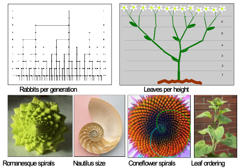
Figure 2.7: Examples of Fibonacci numbers in nature are ubiquitous.

The Fibonacci numbers provide an instructive example of the benefits of dynamic programming. The Fibonacci sequence is recursively defined as F0 = F1 = 1, Fn = Fn−1 + Fn−2 for n ≤ 2. We develop an algorithm to compute the nth Fibonacci number, and then refine it first using memoization and later using dynamic programming to illustrate key concepts.

The Na ̈ıve Solution

The simple top-down approach is to just apply the recursive definition. Listing 1 shows a simple Python implementation.

Listing 2.1: Python implementation for computing Fibonacci numbers recursively.

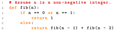
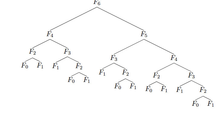
But this top-down algorithm runs in exponential time. That is, if T(n) is how long it takes to compute the n^th Fibonacci number, we have that \(T(n)=T(n-1)+T(n-2)+O(1), \text { so } T(n)=O\left(\phi^{n}\right)\)⁹. The problem is that we are repeating work by solving the same subproblem many times.

Figure 2.8: The recursion tree for the fib procedure showing repeated subproblems. The size of the tree is O(φ(n)), where φ is the golden ratio.

The Memoization Solution

A better solution that still utilizes the top-down approach is to memoize the answers to the subproblems. Listing 2 gives a Python implementation that uses memoization.

Listing 2.2: Python implementation for computing Fibonacci numbers using memoization.

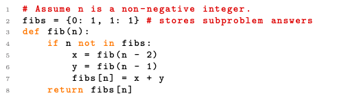
Note that this implementation now runs in T(n) = O(n) time because each subproblem is computed at most once.

The Dynamic Programming Solution

For calculating the nth Fibonacci number, instead of beginning with F(n) and using recursion, we can start computation from the bottom since we know we are going to need all of the subproblems anyway. In this way, we will omit much of the repeated work that would be done by the na ̈ıve top-down approach, and we will be able to compute the nth Fibonacci number in O(n) time.

As a formal exercise, we can apply the steps outlined in section 2.4.1:

1. Find a ’matrix’ parameterization: In this case, the matrix is one-dimensional; there is only one

   parameter to any subproblem F(x).

2. Ensure the subproblem space is polynomial: Since there are only n − 1 subproblems, the space is

   polynomial.

3. Determine an effective transversal order: As mentioned above, we will apply a bottom-up transversal order (that is, compute the subproblems in ascending order).
4. Determine a recursive formula: This is simply the well-known recurrance F(n) = F(n−1)+F(n−2).
5. Remember choices: In this case there is nothing to remember, as no choices were made in the recursive formula.
   Listing 3 shows a Python implementation of this approach.

This method is optimized to only use constant space instead of an entire table since we only need the answer to each subproblem once. But in general dynamic programming solutions, we want to store the solutions to subproblems in a table since we may need to use them multiple times without recomputing their answers. Such solutions would look somewhat like the memoization solution in Listing 2, but they will generally be bottom-up instead of top-down. In this particular example, the distinction between the memoization solution and the dynamic programming solution is minimal as both approaches compute all subproblem solutions and use them the same number of times. In general, memoization is useful when not all subproblems will be computed, while dynamic programming saves the overhead of recursive function calls, and is thus preferable when all subproblem solutions must be calculated¹⁰. Additional dynamic programming examples may be found online [7].

Sequence Alignment using Dynamic Programming

We are now ready to solve the more difficult problem of sequence alignment using dynamic programming, which is presented in depth in the next section. Note that the key insight in solving the sequence alignment problem is that alignment scores are additive. This allows us to create a matrix M indexed by i and j, which are positions in two sequences S and T to be aligned. The best alignment of S and T corresponds with the best path through the matrix M after it is filled in using a recursive formula.

By using dynamic programming to solve the sequence alignment problem, we achieve a provably optimal solution, that is far more efficient than brute-force enumeration.

---

⁹ φ is the golden ratio, i.e. \(\frac{1+\sqrt{5}}{2}\)

¹⁰ In some cases dynamic programming is virtually the only acceptable solution; this is the case in particular when dependency chains between subproblems are long: in this case, the memoization-based solution recurses too deeply, and causes a stack overflow