1.18: Serial Dilutions and Standard Curves with a Microplate Readers

Learning Objectives

Goals:

• Perform several serial dilutions.
• Use spectrophotometry to measure the absorbance of solutions.

Student Learning Outcomes:

Upon completion of this lab, students will be able to:

• Create a series of solutions of decreasing concentrations via serial dilutions.
• Measure the absorbance of solutions with a microplate reader.
• Generate standard curves in Excel.
• Evaluate the quality of standard curves by their R2 value.

Part I: Serial Dilutions

Introduction

A serial dilution is a series of dilutions made sequentially, using the same dilution factor for each step. The concentration factor is the initial volume divided by the final solution volume; the dilution factor would be the inverse of the concentration factor. For example, if you take 1 part of a sample and add 9 parts of water (solvent), then you have made a 1:10 dilution; this is 1/10th (0.1) of the concentration of the original solution and has a dilution factor of 10. These serial dilutions are often used to determine the approximate concentration of an enzyme (or molecule) to be quantified in an assay. Serial dilutions allow for small aliquots to be diluted instead of wasting large quantities of materials, are cost-effective, and are easy to prepare.

Equation 1

\[\text{concentration factor}= \dfrac{\text{volume}_{\text{initial}}}{\text{volume}_{\text{final}}}\nonumber\]

\[\text{dilution factor}= \dfrac{1}{\text{concentration factor}}\nonumber\]

Figure 1. A ten-fold serial dilution, which can also be called a 1:10 dilution, or a series with dilution factor of 10. To determine the concentration at each step of the series, you divide the previous concentration by the dilution factor. *Dilution tubes begin with 9-mL. 1-mL is added and mixed, then 1-mL is transferred to the next tube. The ending volume in the last tube would be 10-mL.

Diagram of 1:2 Serial Dilutions

In your notebook, draw a diagram showing the serial dilutions for the 6 colored solutions you are preparing. In the diagram, indicate the volume being withdrawn from the concentrated solution, the volume of water added, the concentration of the new solution, and the total volume.

Practice Calculations

Problem 1. Assume the original sample used in Figure 1 contained 400 g/L of Reagent X.

1. Then the first 1:10 dilution tube would have a concentration of 400/10 = __________
2. Then the second 1:10 dilution would have a concentration of ____________

Problem 2. Assume the original sample used in Figure is considered 100% concentration.

1. Then the first 1:10 dilution tube would have a _____ % concentration.
2. The second 1:10 dilution tube would have a _____ % concentration.

Problem 3. To make a serial dilution with a dilution factor of 5, you would need to add 1 part of the reagent plus ___ parts of water to make a total of 5 parts. This five-fold serial dilution would have concentrations of 100%, ______% in first diluted tube, _____% in second diluted tube, ________% in third diluted tube.

Problem 4. Suppose the third diluted tube of a two-fold serial dilution has a concentration of 300 g/L.

1. That means that the second diluted tube has a concentration of _________
2. The first diluted tube has a concentration of ________
3. The original tube has a concentration of _______
4. What formula could you use to calculate the concentration of the original tube from the problem statement?

Part 1: Making Serial Dilutions

Materials

Reagents

• Blue (or other color) food dye
• DI H₂O
• 96 well microplate (dry)

Supplies

• P200 Micropipette
• Box of P200 Pipet tips

Note

Use one pipet tip for each serial dilution.

Procedure

Preparing Two-Fold Serial Dilution (Dilution Factor of Two)

1. Obtain a clean, dry 96 well microplate, always touching the edges only. Use a dry clean paper towel to wipe off any fingerprints on the bottom of the plate.
2. Hold plate up to the light and check that there are no dirty spots on the three rows that you will use.
3. (Optional) You can scan the plate with no liquid, to find out the baseline absorbance of the plastic.
4. Pipet 100 µL of DI-water into the first 5 wells of row A (A1-A5).
5. Pipet 100 µL of the original blue dye into the first well (A1). Carefully pipet up and down twice to mix.
6. You do not need to change the pipet tip. But make sure that you released all liquid into the first well.
7. Transfer 100 µL of the mixture into the next well (A2). Mix carefully and release all liquid.
8. Transfer 100 µL of the mixture into the next well (A3). Mix carefully and release all liquid.
9. Transfer 100 µL of the mixture into the next well (A4). Mix carefully and release all liquid.
10. Transfer 100 µL of the mixture into the next well (A5). Mix carefully and release all liquid.
11. Transfer 100 µL of the mixture into the next well (A6). This ensures that all well A1-A5 have the same volume.
12. Take a photo of the wells on top of a white paper.

Preparing Four-Fold Serial Dilution (Dilution Factor of Four)

1. Using a new pipet tip, pipet 150 µL of DI-water into the first 5 wells of row B (B1-B5).
2. You do not need to change the pipet tip. Pipet 50 µL of the original blue dye into the first well (B1). Carefully pipet up and down twice to mix. Then make sure that you released all liquid into the first well.
3. Transfer 50 µL of the mixture into the next well (B2). Mix carefully and release all liquid.
4. Transfer 50 µL of the mixture into the next well (B3). Mix carefully and release all liquid.
5. Transfer 50 µL of the mixture into the next well (B4). Mix carefully and release all liquid.
6. Transfer 50 µL of the mixture into the next well (B5). Mix carefully and release all liquid.
7. Transfer 50 µL of the mixture into the next well (B6). This ensures that all wells B1-B5 have the same volume.
8. Take a photo of the wells on top of a white paper.

Preparing Five-Fold Serial Dilution (Dilution Factor of Five)

1. Using a new pipet tip, pipet 160 µL of DI-water into the first 5 wells of row C (C1-C5).
2. You do not need to change the pipet tip. Pipet 40 µL of the original blue dye into the first well (C1). Carefully pipet up and down twice to mix. Then make sure that you released all liquid into the first well.
3. Transfer 40 µL of the mixture into the next well (C2). Mix carefully and release all liquid.
4. Transfer 40 µL of the mixture into the next well (C3). Mix carefully and release all liquid.
5. Transfer 40 µL of the mixture into the next well (C4). Mix carefully and release all liquid.
6. Transfer 40 µL of the mixture into the next well (C5). Mix carefully and release all liquid.
7. Transfer 40 µL of the mixture into the next well (C6). This ensures that all wells C1-C5 have the same volume.
8. Take a photo of the wells on top of a white paper.

Figure 2: Microplate and serial dilutions.

Part II: Measuring Absorbance

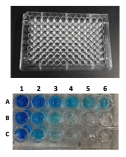
A microplate reader is a spectrophotometric instrument that can measure the absorbance of 96 different samples at one time. Does that save time compared to working with individual cuvettes and a spectrophotometer? We will use a microplate with 96 wells, so that you can perform all of your serial dilutions onto one plate and scan the entire plate with the microplate reader once. The microplate has rows marked A-H and columns marked #1-12. Using blue dye, you will make a 1:2 serial dilution on row A, make a 1:4 serial dilution on row B, and a 1:5 serial dilution on row C.

Materials:

• Equipment
• Microplate Reader and cables
• Laptop computer with program installed to run microplate reader

Procedure:

1. Attach the cable from laptop computer to microplate reader.
2. Power “ON” the laptop computer and the microplate reader.
3. Open the computer program to run the microplate reader.
4. Push the button to open the microplate reader and expose the microplate loading platform.
5. Place your microplate securely into the holder area, ensuring that well A1 is at the top left corner.
6. Push the button to close the microplate reader.
7. On the computer program, start “read new plate” using wavelength 595 nm (for blue dye). You might use a different wavelength if instructed to do to correspond to the best absorbance for the dye you are using.
8. With the computer mouse, highlight the cells corresponding to the microplate wells that you used. Take a photo of the computer screen and note the Absorbance data in the tables below.
9. Calculate the dye concentration for each well, by dividing the dilution factor for each step of the serial dilution. The original dye is 100% concentration.

Data Table 1. Absorbance Measurements of Two-Fold Serial Dilution with Microplate Reader

Well	A1	A2	A3	A4	A5
Absorbance @ 595 nm
Dye Concentration

Data Table 2. Absorbance Measurements of Four-Fold Serial Dilution with Microplate Reader

Well	A1	A2	A3	A4	A5
Absorbance @ 595 nm
Dye Concentration

Data Table 3. Absorbance Measurements of Five-Fold Serial Dilution with Microplate Reader

Well	A1	A2	A3	A4	A5
Absorbance @ 595 nm
Dye Concentration

Part III: Standard Curves

Introduction

Standard curves (also known as calibration curves) show the relationship between two quantities. The standard curves are most often used to determine the concentration of “unknown” samples by comparing them to reference samples with “known” concentrations. Later in the course, we will use standard curves to measure amounts of extracted protein and to determine the size of DNA molecules. In today’s lab, you made three serial dilutions and should be able to calculate the concentrations for each dilution. Using Excel, you will prepare standard curves for each serial dilution and determine if your standard curve is accurate. Then you will determine the concentration of unknown samples, using your standard curves.

Figure 3: Standard curve of a five-fold serial dilution

The R-squared value (R2) is the correlation coefficient or the square of the correlation. For the standard curve, this value measures how strong the linear relationship is between the reagent concentration (X-axis) and the absorbance value (Y-axis). If the R2 value = 1, then that shows a perfect positive relationship. Since your standard curves are generated from the serial dilutions you pipetted, the R2 values can also show how accurate your pipetting skills are.

Activity A: Making a Standard Curve for Each Serial Dilution

1. Enter the data into Excel.
2. Select the data values with your mouse. On the Insert tab, click on the Scatter icon and select Scatter with Straight Lines and Markers from its drop-down menu to generate the standard curve.
3. Be sure to add graph title and labels for X and Y axes.
4. To add a trendline to the graph, right-click on the standard curve line in the chart to display a pop-up menu of plot-related actions. Choose Add Trendline from this menu.
5. Select “display equation on chart” and “display R-squared value on chart”. Ideally, the R2 value should be greater than 0.99.
6. Print the standard curves and add to your notebook.

Activity B: Determining the Concentration of “Unknown” Samples

1. Your instructor will have several unknown samples.
2. Determine the absorbance values of each sample.
3. On your standard curve, use the graph equation to solve for the corresponding concentration of these samples. Or estimate from the line graph.

Data Table 4. Concentration Compared to Serial Dilution Graphs

Unknown Sample	Absorbance	2-fold	4-fold	5-fold

Study Questions

1. Using a serial dilution, describe how you would prepare 10 mL of 1.0%, 0.1% and 0.01% solutions of NaOH. The stock solution is 10% NaOH. Draw diagrams as part of your descriptions/protocols.
2. Using the depicted standard curve, calculate the concentration of an unknown solution if its absorbance value is 0.55.
3. Evaluate the quality of the standard curve (see diagram) by using the R2 value.

Figure 4. Standard curve of absorbance of Copper II