
4.3: Genetic Mapping
- Page ID
- 142555
\( \newcommand{\vecs}[1]{\overset { \scriptstyle \rightharpoonup} {\mathbf{#1}} } \)
\( \newcommand{\vecd}[1]{\overset{-\!-\!\rightharpoonup}{\vphantom{a}\smash {#1}}} \)
\( \newcommand{\dsum}{\displaystyle\sum\limits} \)
\( \newcommand{\dint}{\displaystyle\int\limits} \)
\( \newcommand{\dlim}{\displaystyle\lim\limits} \)
\( \newcommand{\id}{\mathrm{id}}\) \( \newcommand{\Span}{\mathrm{span}}\)
( \newcommand{\kernel}{\mathrm{null}\,}\) \( \newcommand{\range}{\mathrm{range}\,}\)
\( \newcommand{\RealPart}{\mathrm{Re}}\) \( \newcommand{\ImaginaryPart}{\mathrm{Im}}\)
\( \newcommand{\Argument}{\mathrm{Arg}}\) \( \newcommand{\norm}[1]{\| #1 \|}\)
\( \newcommand{\inner}[2]{\langle #1, #2 \rangle}\)
\( \newcommand{\Span}{\mathrm{span}}\)
\( \newcommand{\id}{\mathrm{id}}\)
\( \newcommand{\Span}{\mathrm{span}}\)
\( \newcommand{\kernel}{\mathrm{null}\,}\)
\( \newcommand{\range}{\mathrm{range}\,}\)
\( \newcommand{\RealPart}{\mathrm{Re}}\)
\( \newcommand{\ImaginaryPart}{\mathrm{Im}}\)
\( \newcommand{\Argument}{\mathrm{Arg}}\)
\( \newcommand{\norm}[1]{\| #1 \|}\)
\( \newcommand{\inner}[2]{\langle #1, #2 \rangle}\)
\( \newcommand{\Span}{\mathrm{span}}\) \( \newcommand{\AA}{\unicode[.8,0]{x212B}}\)
\( \newcommand{\vectorA}[1]{\vec{#1}} % arrow\)
\( \newcommand{\vectorAt}[1]{\vec{\text{#1}}} % arrow\)
\( \newcommand{\vectorB}[1]{\overset { \scriptstyle \rightharpoonup} {\mathbf{#1}} } \)
\( \newcommand{\vectorC}[1]{\textbf{#1}} \)
\( \newcommand{\vectorD}[1]{\overrightarrow{#1}} \)
\( \newcommand{\vectorDt}[1]{\overrightarrow{\text{#1}}} \)
\( \newcommand{\vectE}[1]{\overset{-\!-\!\rightharpoonup}{\vphantom{a}\smash{\mathbf {#1}}}} \)
\( \newcommand{\vecs}[1]{\overset { \scriptstyle \rightharpoonup} {\mathbf{#1}} } \)
\(\newcommand{\longvect}{\overrightarrow}\)
\( \newcommand{\vecd}[1]{\overset{-\!-\!\rightharpoonup}{\vphantom{a}\smash {#1}}} \)
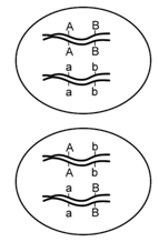
\(\newcommand{\avec}{\mathbf a}\) \(\newcommand{\bvec}{\mathbf b}\) \(\newcommand{\cvec}{\mathbf c}\) \(\newcommand{\dvec}{\mathbf d}\) \(\newcommand{\dtil}{\widetilde{\mathbf d}}\) \(\newcommand{\evec}{\mathbf e}\) \(\newcommand{\fvec}{\mathbf f}\) \(\newcommand{\nvec}{\mathbf n}\) \(\newcommand{\pvec}{\mathbf p}\) \(\newcommand{\qvec}{\mathbf q}\) \(\newcommand{\svec}{\mathbf s}\) \(\newcommand{\tvec}{\mathbf t}\) \(\newcommand{\uvec}{\mathbf u}\) \(\newcommand{\vvec}{\mathbf v}\) \(\newcommand{\wvec}{\mathbf w}\) \(\newcommand{\xvec}{\mathbf x}\) \(\newcommand{\yvec}{\mathbf y}\) \(\newcommand{\zvec}{\mathbf z}\) \(\newcommand{\rvec}{\mathbf r}\) \(\newcommand{\mvec}{\mathbf m}\) \(\newcommand{\zerovec}{\mathbf 0}\) \(\newcommand{\onevec}{\mathbf 1}\) \(\newcommand{\real}{\mathbb R}\) \(\newcommand{\twovec}[2]{\left[\begin{array}{r}#1 \\ #2 \end{array}\right]}\) \(\newcommand{\ctwovec}[2]{\left[\begin{array}{c}#1 \\ #2 \end{array}\right]}\) \(\newcommand{\threevec}[3]{\left[\begin{array}{r}#1 \\ #2 \\ #3 \end{array}\right]}\) \(\newcommand{\cthreevec}[3]{\left[\begin{array}{c}#1 \\ #2 \\ #3 \end{array}\right]}\) \(\newcommand{\fourvec}[4]{\left[\begin{array}{r}#1 \\ #2 \\ #3 \\ #4 \end{array}\right]}\) \(\newcommand{\cfourvec}[4]{\left[\begin{array}{c}#1 \\ #2 \\ #3 \\ #4 \end{array}\right]}\) \(\newcommand{\fivevec}[5]{\left[\begin{array}{r}#1 \\ #2 \\ #3 \\ #4 \\ #5 \\ \end{array}\right]}\) \(\newcommand{\cfivevec}[5]{\left[\begin{array}{c}#1 \\ #2 \\ #3 \\ #4 \\ #5 \\ \end{array}\right]}\) \(\newcommand{\mattwo}[4]{\left[\begin{array}{rr}#1 \amp #2 \\ #3 \amp #4 \\ \end{array}\right]}\) \(\newcommand{\laspan}[1]{\text{Span}\{#1\}}\) \(\newcommand{\bcal}{\cal B}\) \(\newcommand{\ccal}{\cal C}\) \(\newcommand{\scal}{\cal S}\) \(\newcommand{\wcal}{\cal W}\) \(\newcommand{\ecal}{\cal E}\) \(\newcommand{\coords}[2]{\left\{#1\right\}_{#2}}\) \(\newcommand{\gray}[1]{\color{gray}{#1}}\) \(\newcommand{\lgray}[1]{\color{lightgray}{#1}}\) \(\newcommand{\rank}{\operatorname{rank}}\) \(\newcommand{\row}{\text{Row}}\) \(\newcommand{\col}{\text{Col}}\) \(\renewcommand{\row}{\text{Row}}\) \(\newcommand{\nul}{\text{Nul}}\) \(\newcommand{\var}{\text{Var}}\) \(\newcommand{\corr}{\text{corr}}\) \(\newcommand{\len}[1]{\left|#1\right|}\) \(\newcommand{\bbar}{\overline{\bvec}}\) \(\newcommand{\bhat}{\widehat{\bvec}}\) \(\newcommand{\bperp}{\bvec^\perp}\) \(\newcommand{\xhat}{\widehat{\xvec}}\) \(\newcommand{\vhat}{\widehat{\vvec}}\) \(\newcommand{\uhat}{\widehat{\uvec}}\) \(\newcommand{\what}{\widehat{\wvec}}\) \(\newcommand{\Sighat}{\widehat{\Sigma}}\) \(\newcommand{\lt}{<}\) \(\newcommand{\gt}{>}\) \(\newcommand{\amp}{&}\) \(\definecolor{fillinmathshade}{gray}{0.9}\)In the preceding examples, we had the advantage of knowing the approximate chromosomal positions of each allele involved, before we calculated the recombination frequencies. Knowing this information beforehand made it relatively easy to define the parental and recombinant genotypes, and to calculate recombination frequencies. However, in most experiments, we cannot directly examine the chromosomes, or even the gametes, so we must infer the arrangement of alleles from the phenotypes over two or more generations. Importantly, it is generally not sufficient to know the genotype of individuals in just one generation; for example, given an individual with the genotype AaBb, we do not know from the genotype alone whether the loci are located on the same chromosome, and if so, whether the arrangement of alleles on each chromosome is AB and ab or Ab and aB (Figure \(\PageIndex{6}\)). The top cell has the two dominant alleles together and the two recessive alleles together and is said to have the genes in the cis configuration. The alternative shown in the cell below is that the genes are in the trans configuration.
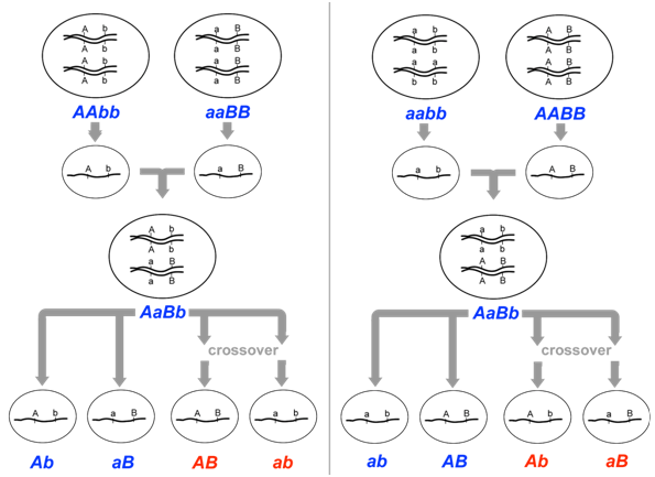
Fortunately for geneticists, the arrangement of alleles can sometimes be inferred if the genotypes of a previous generation are known. For example, if the parents of AaBb had genotypes AABB and aabb respectively, then the parental gametes that fused to produce AaBb would have been genotype AB and genotype ab. Therefore, prior to meiosis in the dihybrid, the arrangement of alleles would likewise be AB and ab (Figure \(\PageIndex{7}\)). Conversely, if the parents of AaBb had genotypes aaBB and AAbb, then the arrangement of alleles on the chromosomes of the dihybrid would be aB and Ab. Thus, the genotype of the previous generation can determine which of an individual’s gametes are considered recombinant, and which are considered parental.
Let us now consider a complete experiment in which our objective is to measure recombination frequency (Figure \(\PageIndex{8}\)). We need at least two alleles for each of two genes, and we must know which combinations of alleles were present in the parental gametes. The simplest way to do this is to start with pure-breeding lines that have contrasting alleles at two loci. For example, we could cross short-tailed mice, brown mice (aaBB) with long-tailed, white mice (AAbb). Based on the genotypes of the parents, we know that the parental gametes will be aB or Ab (but not ab or AB), and all of the progeny will be dihybrids, AaBb. We do not know at this point whether the two loci are on different pairs of homologous chromosomes, or whether they are on the same chromosome, and if so, how close together they are.
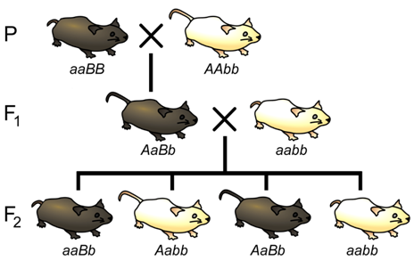
The recombination events that may be detected will occur during meiosis in the dihybrid individual. If the loci are completely or partially linked, then prior to meiosis, alleles aB will be located on one chromosome, and alleles Ab will be on the other chromosome (based on our knowledge of the genotypes of the gametes that produced the dihybrid). Thus, recombinant gametes produced by the dihybrid will have the genotypes ab or AB, and non-recombinant (i.e. parental) gametes will have the genotypes aB or Ab.
How do we determine the genotype of the gametes produced by the dihybrid individual? The most practical method is to use a testcross (Figure \(\PageIndex{8}\)), in other words to mate AaBb to an individual that has only recessive alleles at both loci (aabb). This will give a different phenotype in the F2 generation for each of the four possible combinations of alleles in the gametes of the dihybrid. We can then infer unambiguously the genotype of the gametes produced by the dihybrid individual, and therefore calculate the recombination frequency between these two loci. For example, if only two phenotypic classes were observed in the F2 (i.e. short tails and brown fur (aaBb), and white fur with long tails (Aabb) we would know that the only gametes produced following meiosis of the dihybrid individual were of the parental type: aB and Ab, and the recombination frequency would therefore be 0%. Alternatively, we may observe multiple classes of phenotypes in the F2 in ratios such as shown in Table \(\PageIndex{1}\):
|
tail phenotype |
fur phenotype |
number of progeny |
gamete from dihybrid |
genotype of F2 from test cross |
(P)arental or (R)ecombinant |
|
short |
brown |
48 |
aB |
aaBb |
P |
|
long |
white |
42 |
Ab |
Aabb |
P |
|
short |
white |
13 |
ab |
aabb |
R |
|
long |
brown |
17 |
AB |
AaBb |
R |
Given the data in Table \(\PageIndex{1}\), the calculation of recombination frequency is straightforward:
\[\begin{align} \textrm{recombination frequency} &= \mathrm{\dfrac{number\: of\: recombinant\: gametes}{total\: number\: of\: gametes\: scored}}\\ \textrm{R.F.} &= \dfrac{13+17}{48+42+13+17}\\ &=25\% \end{align}\]
Because the frequency of recombination between two loci (up to 50%) is roughly proportional to the chromosomal distance between them, we can use recombination frequencies to produce genetic maps of all the loci along a chromosome and ultimately in the whole genome. The units of genetic distance are called map units (mu) or centiMorgans (cM), in honor of Thomas Hunt Morgan by his student, Alfred Sturtevant, who developed the concept. Geneticists routinely convert recombination frequencies into cM: the recombination frequency in percent is approximately the same as the map distance in cM. For example, if two loci have a recombination frequency of 25% they are said to be ~25cM apart on a chromosome (Figure \(\PageIndex{9}\)). Note: this approximation works well for small distances (RF<30%) but progressively fails at longer distances because the RF reaches a maximum at 50%. Some chromosomes are >100 cM long but loci at the tips only have an RF of 50%. The method for mapping of these long chromosomes is shown below.
Note that the map distance of two loci alone does not tell us anything about the orientation of these loci relative to other features, such as centromeres or telomeres, on the chromosome.

Map distances are always calculated for one pair of loci at a time. However, by combining the results of multiple pairwise calculations, a genetic map of many loci on a chromosome can be produced (Figure \(\PageIndex{10}\)). A genetic map shows the map distance, in cM, that separates any two loci, and the position of these loci relative to all other mapped loci. The genetic map distance is roughly proportional to the physical distance, i.e. the amount of DNA between two loci. For example, in Arabidopsis, 1.0 cM corresponds to approximately 150,000bp and contains approximately 50 genes. The exact number of DNA bases in a cM depends on the organism, and on the particular position in the chromosome; some parts of chromosomes (“crossover hot spots”) have higher rates of recombination than others, while other regions have reduced crossing over and often correspond to large regions of heterochromatin.

When a novel gene or locus is identified by mutation or polymorphism, its approximate position on a chromosome can be determined by crossing it with previously mapped genes, and then calculating the recombination frequency. If the novel gene and the previously mapped genes show complete or partial linkage, the recombination frequency will indicate the approximate position of the novel gene within the genetic map. This information is useful in isolating (i.e. cloning) the specific fragment of DNA that encodes the novel gene, through a process called map-based cloning.
Genetic maps are also useful to track genes/alleles in breeding crops and animals, in studying evolutionary relationships between species, and in determining the causes and individual susceptibility of some human diseases.

Genetic maps are useful for showing the order of loci along a chromosome, but the distances are only an approximation. The correlation between recombination frequency and actual chromosomal distance is more accurate for short distances (low RF values) than long distances. Observed recombination frequencies between two relatively distant markers tend to underestimate the actual number of crossovers that occurred. This is because as the distance between loci increases, so does the possibility of having a second (or more) crossovers occur between the loci. This is a problem for geneticists, because with respect to the loci being studied, these double-crossovers produce gametes with the same genotypes as if no recombination events had occurred (Figure \(\PageIndex{11}\)) – they have parental genotypes. Thus a double crossover will appear to be a parental type and not be counted as a recombinant, despite having two (or more) crossovers. Geneticists will sometimes use specific mathematical formulae to adjust large recombination frequencies to account for the possibility of multiple crossovers and thus get a better estimate of the actual distance between two loci.
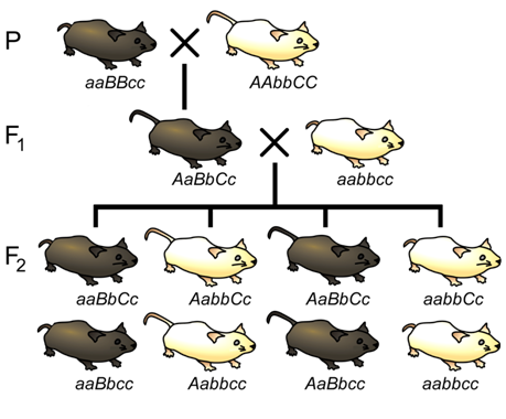
A particularly efficient method of mapping three genes at once is the three-point cross, which allows the order and distance between three potentially linked genes to be determined in a single cross experiment (Figure \(\PageIndex{12}\)). This is particularly useful when mapping a new mutation with an unknown location to two previously mapped loci. The basic strategy is the same as for the dihybrid mapping experiment; pure breeding lines with contrasting genotypes are crossed to produce an individual heterozygous at three loci (a trihybrid), which is then testcrossed to determine the recombination frequency between each pair of genes.
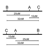
One useful feature of the three-point cross is that the order of the loci relative to each other can usually be determined by a simple visual inspection of the F2 segregation data. If the genes are linked, there will often be two phenotypic classes that are much more infrequent than any of the others. In these cases, the rare phenotypic classes are usually those that arose from two crossover events, in which the locus in the middle is flanked by a crossover on either side of it. Thus, among the two rarest recombinant phenotypic classes, the one allele that differs from the other two alleles relative to the parental genotypes likely represents the locus that is in the middle of the other two loci. For example, based on the phenotypes of the pure-breeding parents in Figure \(\PageIndex{12}\), the parental genotypes are aBC and AbC (remember the order of the loci is unknown, and it is not necessarily the alphabetical order in which we wrote the genotypes). Because we can deduce from the outcome of the testcross (Table \(\PageIndex{2}\)) that the rarest genotypes were abC and ABc, we can conclude that locus A that is most likely located between the other two loci, since it would require a recombination event between both A and B and between A and C in order to generate these gametes. Thus, the order of loci is BAC (which is equivalent to CAB).
|
tail phenotype |
fur phenotype |
whisker phenotype |
number of progeny |
gamete from trihybrid |
genotype of F2 from test cross |
loci A, B |
loci A, C |
loci B, C |
|---|---|---|---|---|---|---|---|---|
|
short |
brown |
long |
5 |
aBC |
aaBbCc |
P |
R |
R |
|
long |
white |
long |
38 |
AbC |
AabbCc |
P |
P |
P |
|
short |
white |
long |
1 |
abC |
aabbCc |
R |
R |
P |
|
long |
brown |
long |
16 |
ABC |
AaBbCc |
R |
P |
R |
|
short |
brown |
short |
42 |
aBc |
aaBbcc |
P |
P |
P |
|
long |
white |
short |
5 |
Abc |
Aabbcc |
P |
R |
R |
|
short |
white |
short |
12 |
abc |
aabbcc |
R |
P |
R |
|
long |
brown |
short |
1 |
ABc |
AaBbcc |
R |
R |
P |
Recombination frequencies may be calculated for each pair of loci in the three-point cross as we did before for one pair of loci in our dihybrid (Figure 7. 8).
\[\begin{alignat}{2} \textrm{loci A,B R.F.} = &\dfrac{1+16+12+1}{120} &&= 25\%\\ \textrm{loci A,C R.F.} = &\dfrac{1+5+1+5}{120} &&= 10\%\\ \textrm{loci B,C R.F.} = &\dfrac{5+16+12+5}{120} &&= 32\%\\ \textrm{(not corrected for double}\\ \textrm{crossovers)}\hspace{40px} \end{alignat}\]
However, note that in the three point cross, the sum of the distances between A-B and A-C (35%) is less than the distance calculated for B-C (32%)(Figure \(\PageIndex{13}\)). this is because of double crossovers between B and C, which were undetected when we considered only pairwise data for B and C. We can easily account for some of these double crossovers, and include them in calculating the map distance between B and C, as follows. We already deduced that the map order must be BAC (or CAB), based on the genotypes of the two rarest phenotypic classes in Table \(\PageIndex{2}\). However, these double recombinants, ABc and abC, were not included in our calculations of recombination frequency between loci B and C. If we included these double recombinant classes (multiplied by 2, since they each represent two recombination events), the calculation of recombination frequency between B and C is as follows, and the result is now more consistent with the sum of map distances between A-B and A-C.
\[\begin{align} \textrm{loci B,C R.F.} &= \dfrac{5+16+12+5+2(1)+2(1)}{120} = 35\%\\ \textrm{(corrected for double}&\\ \textrm{recombinants)}& \end{align}\]
Thus, the three point cross was useful for:
- determining the order of three loci relative to each other,
- calculating map distances between the loci, and
- detecting some of the double crossover events that would otherwise lead to an underestimation of map distance.
However, it is possible that other, double crossovers events remain undetected, for example double crossovers between loci A,B or between loci A,C. Geneticists have developed a variety of mathematical procedures to try to correct for things like double crossovers during large-scale mapping experiments.
As more and more genes are mapped a better genetic map can be constructed. Then, when a new gene is discovered, it can be mapped relative to other genes of known location to determine its location. All that is needed to map a gene is two alleles, a wild type allele (e.g. A) and a mutant allele (e.g. 'a').