2.2.2: Tandem Repeats and PCR

What is a tandem repeat?

A tandem repeat is a region of the genome where a short nucleotide sequence (from two bases to several hundred bases) is repeated one-after-another -- that is, "in tandem." Various types of tandem repeats have been described:

• Microsatellites are tandem repeats of two to six bases, typically repeated 5 to 50 times. They are also sometimes called short tandem repeats (STRs) and simple sequence repeats (SSRs).
• Minisatellites are tandem repeates where a DNA motif of 10 to 50 bases is repeated from two to several hundred times. 

Tandem repeats are useful molecular markers because they are hypervariable - due to errors during replication, they readily gain or lose repeats. As indicated at the end of the previous section, this can lead to an RFLP polymorphism. However, more sophisticated methods allow researchers to genotype tandem repeats very accurately from very small amounts of DNA. This is particularly useful for crime scene analysis! There are two key methods -- PCR and capillary electrophoresis.

Polymerase Chain Reaction (PCR)

Most methods of DNA analysis, such as restriction enzyme digestion and agarose gel electrophoresis, or DNA sequencing require large amounts of a specific DNA fragment. In the past, large amounts of DNA were produced by growing the host cells of a genomic library. However, libraries take time and effort to prepare and DNA samples of interest often come in minute quantities. The polymerase chain reaction (PCR) permits rapid amplification in the number of copies of specific DNA sequences for further analysis (Figure \(\PageIndex{8}\)). One of the most powerful techniques in molecular biology, PCR was developed in 1983 by Kary Mullis while at Cetus Corporation. PCR has specific applications in research, forensic, and clinical laboratories, including:

• determining the sequence of nucleotides in a specific region of DNA
• amplifying a target region of DNA for cloning into a plasmid vector
• identifying the source of a DNA sample left at a crime scene
• analyzing samples to determine paternity
• comparing samples of ancient DNA with modern organisms
• determining the presence of difficult to culture, or unculturable, microorganisms in humans or environmental samples

PCR is an in vitro laboratory technique that takes advantage of the natural process of DNA replication. The heat-stable DNA polymerase enzymes used in PCR are derived from hyperthermophilic prokaryotes. Taq DNA polymerase, commonly used in PCR, is derived from the Thermus aquaticus bacterium isolated from a hot spring in Yellowstone National Park. DNA replication requires the use of primers for the initiation of replication to have free 3ʹ-hydroxyl groups available for the addition of nucleotides by DNA polymerase. However, while primers composed of RNA are normally used in cells, DNA primers are used for PCR. DNA primers are preferable due to their stability, and DNA primers with known sequences targeting a specific DNA region can be chemically synthesized commercially. These DNA primers are functionally similar to the DNA probes used for the various hybridization techniques described earlier, binding to specific targets due to complementarity between the target DNA sequence and the primer.

PCR occurs over multiple cycles, each containing three steps: denaturation, annealing, and extension. Machines called thermal cyclers are used for PCR; these machines can be programmed to automatically cycle through the temperatures required at each step (Figure 12.1). First, double-stranded template DNA containing the target sequence is denatured at approximately 95 °C. The high temperature required to physically (rather than enzymatically) separate the DNA strands is the reason the heat-stable DNA polymerase is required. Next, the temperature is lowered to approximately 50 °C. This allows the DNA primers complementary to the ends of the target sequence to anneal (stick) to the template strands, with one primer annealing to each strand. Finally, the temperature is raised to 72 °C, the optimal temperature for the activity of the heat-stable DNA polymerase, allowing for the addition of nucleotides to the primer using the single-stranded target as a template. Each cycle doubles the number of double-stranded target DNA copies. Typically, PCR protocols include 25–40 cycles, allowing for the amplification of a single target sequence by tens of millions to over a trillion.

Natural DNA replication is designed to copy the entire genome, and initiates at one or more origin sites. Primers are constructed during replication, not before, and do not consist of a few specific sequences. PCR targets specific regions of a DNA sample using sequence-specific primers. In recent years, a variety of isothermal PCR amplification methods that circumvent the need for thermal cycling have been developed, taking advantage of accessory proteins that aid in the DNA replication process. As the development of these methods continues and their use becomes more widespread in research, forensic, and clinical labs, thermal cyclers may become obsolete.

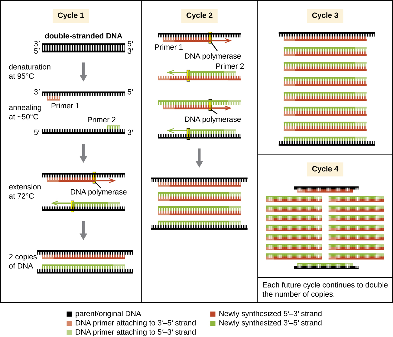
Figure \(\PageIndex{8}\): The polymerase chain reaction (PCR) is used to produce many copies of a specific sequence of DNA.

 

Capillary Electrophoresis 

Imagine you have used PCR to amplify a microsatellite, and you know that it may have 14 or 15 copies of a three-base-pair motif. Are you going to be able to tell which allele you are looking at on an agarose gel? No!

Enter capillary electrophoresis (CE). A CE instrument separates DNA molecules using a polymer in a long, thin capillary tube. For reasons that are beyond the scope of this explanation, it is much more sensitive than agarose gel electrophoresis -- CE can reliably separate DNA molecules that differ by only one base! As a result, CE can be used to analyse microsatellites that are amplified with PCR:

 

Figure \(\PageIndex{9}\): Short tandem repeat (STR) analysis on a simplified model using polymerase chain reaction (PCR): First, a DNA sample undergoes PCR with primers targeting certain STRs (which vary in lengths between individuals and their alleles). The resultant fragments are separated by size (such as electrophoresis). (Source: Wikipedia, Mikael Haggstrom, MD. CC-BY.)

Another useful attribute of this type of genotyping is that you can multiplex it -- a single PCR reaction with multiple sets of primers can give the genotypes of multiple sites with a single PCR and a single run on a CE instrument. For example, the following image shows a person's genotype at 7 microsatellite loci. (The loci names are in the grey boxes above the electrophoretogram.) The genotyped individual is heterozygous at six. At which locus are they homozygous? How do you know?

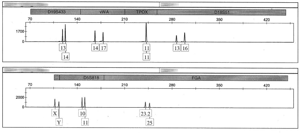
Figure \(\PageIndex{9}\): Str profile. Bottom two lines (yellow and red dyes) of a human genetic profile typed using Applied Biosystems' Identifiler kit when viewed in GeneMapper ID. The X-axis represents the length of the STR fragments, the Y-axis is the intensity of the signal. This is my own profile, so there are no privacy issues in uploading this image. Source: Sekiyu at the English language Wikipedia. CC BY-SA.