4: Semelparity versus Iteroparity

Semelparity versus Iteroparity

Semelparity and iteroparity are two contrasting reproductive strategies available to living organisms. A species is considered semelparous if it is characterized by a single reproductive episode before death, and iteroparous if it is characterized by multiple reproductive cycles over the course of its lifetime.

In truly semelparous species, death after reproduction is part of an overall strategy that includes putting all available resources into maximizing reproduction, at the expense of future life. In any iteroparous population there will be some individuals who die between their first and second reproductive episodes, but unless this is part of a syndrome of programmed death after reproduction, this would not be called semelparity.

This distinction is also related to the difference between annual and perennial plants. An annual is a plant that completes its life cycle in a single season, and is usually semelparous. Perennials live for more than one season and are usually (but not always) iteroparous.^[1]

Semelparity and iteroparity are not, strictly speaking, alternative strategies, but extremes along a continuum of possible modes of reproduction. Many organisms considered to be semelparous can, under certain conditions, separate their single bout of reproduction into two or more episodes.^[2][3]

 

Semelparity

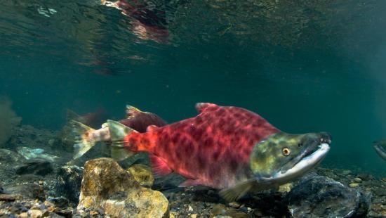
The word semelparity was coined by evolutionary biologist Lamont Cole^[4], and comes from the Latin semel 'once, a single time' and pario 'to beget'. This differs from iteroparity in that iteroparous species are able to have multiple reproductive cycles and therefore can mate more than once in their lifetime. Semelparity is also known as "big bang" reproduction, since the single reproductive event of semelparous organisms is usually large as well as fatal^[5]. A classic example of a semelparous organism is Pacific salmon (Oncorhynchus spp.), which lives for many years in the ocean before swimming to the freshwater stream of its birth, spawning, and dying. Other semelparous animals include many insects, including some species of butterflies, cicadas, and mayflies, many arachnids, and some molluscs such as some species of squid and octopus. Annual plants, including all grain crops and most domestic vegetables, are semelparous. Long-lived semelparous plants include century plant (agave), Lobelia telekii, and some species of bamboo.

Figure \(\PageIndex{1}\): Many Pacific salmon, like this sockeye salmon (Oncorhynchus nerka) are semelparous and only reproduce once in their lifetime. Source: Milton Love, Marine Science Institute, available in the public domain.

This form of lifestyle is consistent with r-selected strategies as many offspring are produced and there is low parental input, as one or both parents die after mating. All of the male’s energy is diverting into mating and the immune system is repressed. High levels of corticosteroids are sustained over long periods of time. This triggers immune and inflammatory system failure and gastrointestinal hemorrhage, which eventually leads to death.

 

Iteroparity

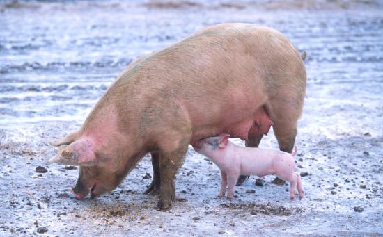
The term iteroparity comes from the Latin itero, to repeat, and pario, to beget. An example of an iteroparous organism is a human—humans are biologically capable of having offspring many times over the course of their lives. Iteroparous vertebrates include all birds, most reptiles, virtually all mammals, and most fish. Among invertebrates, most mollusca and many insects (for example, mosquitoes and cockroaches) are iteroparous. Most perennial plants are iteroparous.

Figure \(\PageIndex{2}\): Most mammals, like this domestic pig are iteroparous and reproduce multiple times in their life. Source: Scott Bauer, USDA, available in the public domain.

 

Trade-offs

Within its lifetime, an organism has a limited amount of energy/resources available to it and must always partition it among various functions such as collecting food and finding a mate. Of relevance here is the trade-off between fecundity, growth, and survivorship in its life history strategy. These trade-offs come into play in the evolution of iteroparity and semelparity. It has been repeatedly demonstrated that semelparous species produce more offspring in their single fatal reproductive episode than do closely related iteroparous species in any one of theirs. However, the opportunity to reproduce more than once in a lifetime, and possibly with greater care for the development of offspring produced, can offset this strictly numerical benefit.

 

Models based on non-linear trade-offs

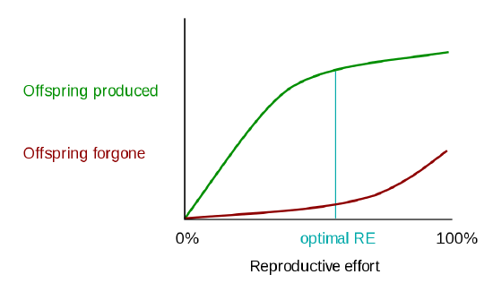
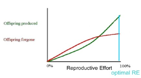
One class of models that tries to explain the differential evolution of semelparity and iteroparity examines the shape of the trade-off between offspring produced and offspring forgone (offspring that will not be produced). In economic terms, offspring produced is equivalent to a benefit function, while offspring forgone is comparable to a cost function. The reproductive effort of an organism—the proportion of energy that it puts into reproducing, as opposed to growth or survivorship—occurs at the point where the distance between offspring produced and offspring forgone is the greatest (Figure 3).

Figure \(\PageIndex{3}\): A visual model to explain the evolution of semelparity and iteroparity based on different cost/benefit curves. In the first graph, the marginal cost of offspring produced is decreasing (each additional offspring is less "expensive" than the average of all previous offspring) and the marginal cost of offspring forgone is increasing. In this situation, the organism only devotes a portion of its resources to reproduction, and uses the rest of its resources on growth and survivorship so that it can reproduce again in the future^[6]. However, it is also possible (second graph) for the marginal cost of offspring produced to increase, and for the marginal cost of offspring forgone to decrease. When this is the case, it is favorable for the organism to reproduce a single time. The organism devotes all of its resources to that one episode of reproduction, so it then dies. This mathematical/graphical model has found only limited quantitative support from nature. Source: Paul Moorcroft, Harvard University, licensed under CC BY-SA 3.0.

 

Bet-hedging models

A second set of models examines the possibility that iteroparity is a hedge against unpredictable juvenile survivorship (avoiding putting all one's eggs in one basket). Again, mathematical models have not found empirical support from real-world systems. In fact, many semelparous species live in habitats characterized by high (not low) environmental unpredictability, such as deserts and early successional habitats.

 

Cole's paradox and demographic models

The models that have the strongest support from living systems are demographic. In Lamont Cole's classic 1954 paper, he came to the conclusion that: "For an annual species, the absolute gain in intrinsic population growth which could be achieved by changing to the perennial reproductive habit would be exactly equivalent to adding one individual to the average litter size." ^[7]

For example, imagine two species—an iteroparous species that has annual litters averaging three offspring each, and a semelparous species that has one litter of four, and then dies. These two species have the same rate of population growth, which suggests that even a tiny fecundity advantage of one additional offspring would favor the evolution of semelparity. This is known as Cole's paradox. In his analysis, Cole assumed that there was no mortality of individuals of the iteroparous species, even seedlings. Twenty years later, Charnov and Schaffer^[8] showed that reasonable differences in adult and juvenile mortality yield much more reasonable costs of semelparity, essentially solving Cole's paradox. An even more general demographic model was produced by Young^[9]. These demographic models have been more successful than the other models when tested with real-world systems. It has been shown that semelparous species have higher expected adult mortality, making it more economical to put all reproductive effort into the first (and therefore final) reproductive episode.^[10][11]

 

Sources  

1.  Gotelli, N.J. (2008). A primer of ecology. Sunderland, Mass.: Sinauer Associates, Inc. ISBN 978-0-87893-318-1
2. Futami, K., & Akimoto, S. (2005). Facultative second oviposition as an adaptation to egg loss in a semelparous crab spider. Etholgy, 111(12), pp. 1126-1138. Bibcode:2005Ethol.111.1126F. doi:10.1111/j.1439-0310.2005.01126.x. ISSN 1439-0310.
3. Hughes, P.W., & Simons, A.M. (2014). Changing reproductive effort within a semelparous reproductive episode. American Journal of Botany, 101(8), pp. 1323-1331. doi:10.3732/ajb.1400283. ISSN 0002-9122. PMID 25156981.
4. Cole, L.C. (1954). The population consequences of life history phenomena. The Quarterly Review of Biology, 29(2), pp. 103-137. doi:10.1086/400074. JSTOR 2817654. PMID 13177850. S2CID 26986186.
5. Ricklefs, R.E., & Miller, G.L. (1999). Ecology. Macmillan ISBN 0-7167-2829-X
6. Roff, D.A. (1992). The evolution of life histories. Springer ISBN 0-412-02391-1
7. Lamont, C.C. (1954). The population consequences of life history phenomena. The Quarterly Review of Biology, 29(2), pp. 103-137.
8. Charnov, E.L., & Schaffer, W.M. (1973). Life history consequences of natural selection: Cole's result revisited. American Naturalist, 107(958), pp. 791-793. doi:10.1086/282877. S2CID 83561052.
9. Young, T.P. (1981). A general mode of comparative fecundity for semelparous and iteroparous life histories. American Naturalist, 118, pp. 27-36. doi:10.1086/283798. S2CID 83860904.
10. Young, T.P. (1990). The evolution of semelparity in Mount Kenya lobelias. Evolutionary Ecology, 4(2), pp. 157-171. doi:10.1007/bf02270913. S2CID 25993809.
11. Lesica, P., & Young, T.P. (2005). Demographic model explains life history evolution in Arabis fecunda. Functional Ecology, 19(3), pp. 471-477. doi:10.1111/j.1365-2435.2005.00972.x. S2CID 31222891.

 

Contributors and Attributions  

This chapter was written by D. Wetzel with text taken from the following CC-BY resources:

• Wikipedia: https://en.wikipedia.org/wiki/Semelparity_and_iteroparity