4.7: Biomolecular Visualization - Conceptions and Misconceptions

Search Fundamentals of Biochemistry

Learning Goals 

(Learning goals written by Claude, Sonnet 4.6, Anthropic)

Principles of Molecular Visualization

• Explain the physical basis and key limitations of structural data from X-ray crystallography and cryo-EM — including the absence of hydrogen atoms, the static nature of a single conformer from a dynamic ensemble, and the potential for modeling errors — and describe how these limitations affect the interpretation of bond connectivity, geometry, and noncovalent interactions displayed in computer models.
• Select and justify the most appropriate molecular rendering (line, stick, ball-and-stick, spacefill, surface, or cartoon) for a given structural question, explaining what each representation reveals and conceals about atom connectivity, relative atomic size, steric accessibility, and secondary structure.

Applying Renderings to Infer Structure-Function Relationships

• Interpret spacefill and van der Waals surface renderings to assess steric effects, molecular shape, and packing density in both small molecules (e.g., oleic acid) and large ones (e.g., proteins), and explain why line or stick renderings alone are insufficient for understanding how atomic size influences structure and reactivity.
• Interpret an electrostatic potential surface map — in which red regions indicate high electron density (partial or full negative charge) and blue regions indicate low electron density (partial or full positive charge) — and use this rendering to predict how charge distribution directs substrate binding, as illustrated by the positively charged active-site channel of superoxide dismutase attracting the negatively charged superoxide radical O₂⁻.
• Explain how cartoon representations of proteins — displaying α-helices as ribbons or cylinders, β-strands as arrows, and loops as tubes — reveal secondary structure organization and overall topology while necessarily omitting side chain information, and describe when mixed renderings (cartoon plus stick side chains, or surface plus cartoon) provide the most complete structural insight.

Structure determines everything in biology and chemistry. Since you learned to represent molecules with Lewis structures, it's been drilled into you that the structure of a molecule determines its physical and chemical properties. Physical properties would include melting points, boiling points, and solubility. In contrast, chemical properties include acid/base, redox, precipitation, and general chemical reactivity determined by the presence of Lewis/Brønsted acids/bases and nucleophiles/electrophiles. More modern analyses of reactivity would include molecular orbital theory descriptions of bonding.

We can't see molecules but make inferences from data (x-ray crystallography, NMR spectroscopy, and cryo-EM) about the structure of a molecule (atom type, atom/bond connectivity, and geometry). As molecules get larger (consider the muscle protein titin, also called connectin, with a molecular weight of around 3.8 million), we must use computer visualization to understand its structure and infer its resulting function and activity. As with small molecules, we can render the molecule in different ways to better understand the attributes that confer function and activity. We ask students to view a biomolecule and infer its properties from the rendering, without giving them dedicated attention or instruction on how to do so.

Small molecules

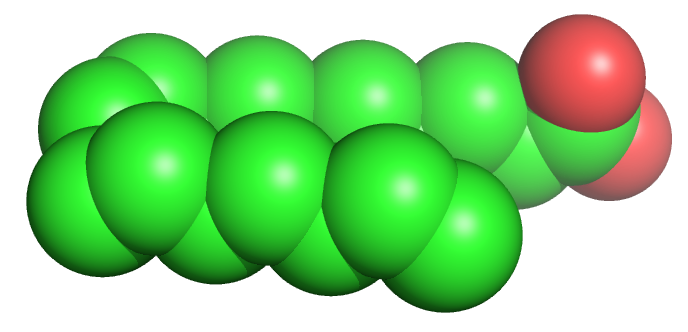
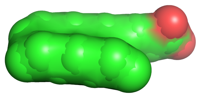
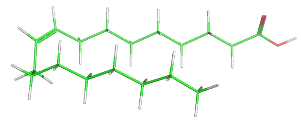
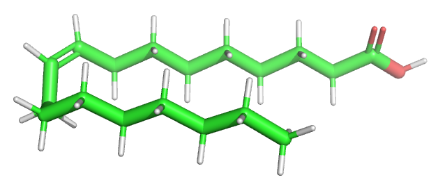
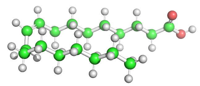
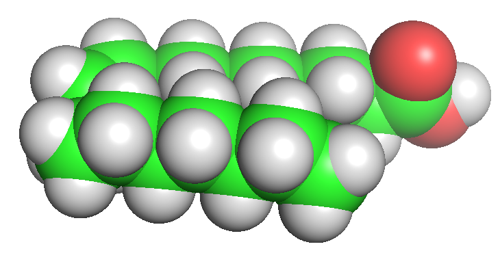
Let's start with a small molecule like oleic acid, a long chain carboxylic acid with 18 carbon atoms and one cis (Z) double bond between carbons 9 and 10, as shown in Figure \(\PageIndex{1}\).

Figure \(\PageIndex{1}\): Line drawing of oleic acid

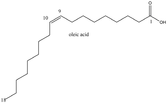
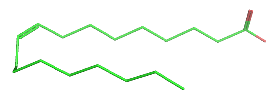
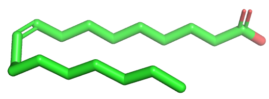
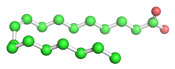
Table \(\PageIndex{1}\) below shows multiple ways to render the molecule. Each rendering offers insight into the molecule's function/activity but might, at the same time, leave students struggling to interpret it, reinforcing or instilling misconceptions. Each representation below shows the very same molecule. The top row shows representations without H atoms; the bottom row shows those with H atoms.

line	stick	ball sphere	sphere	surface

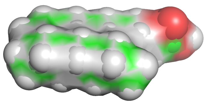Table \(\PageIndex{1}\):Different renderings of oleic acid

Here are some important things to remember about biomolecular structures, including both small and large molecules:

• Structures obtained using X-ray crystallography are constructed from relative electron densities calculated from diffraction patterns. Computer programs calculate the structure based on these electron density maps and known bond lengths, bond angles, and atom types. Most of the structures used in this book are available in the Protein Data Bank. The structures seen in computer models are visualized data and may contain errors (missing atoms, steric clashes, incorrect atom assignments), although structural refinement techniques minimize such problems.
• Structures derived from X-ray and cryomicroscopy analyses are static and represent only one conformation from a large ensemble. As you learned from studying simple molecules in organic chemistry, bond length and angle changes continually occur within molecules. Bonds connecting two atoms can stretch, angles connecting three atoms can bend, and the torsional angle around the center bond in a four-atom, three-bond system can rotate to form eclipsed and staggered (gauche and anti) conformers.
• PDB structures obtained by X-ray crystallography contain no H atoms as they are too small and contain too few electrons to diffract/scatter X-rays. So get used to adding them in your mind when you see a structure. Programs are used to calculate and show H bonds between a slightly positive H atom on an O or N atom in a protein and another slightly negative Os or Ns on the same or different molecule. The H bonds are often shown between N and O atoms. You should look at the atoms involved and the distance between them, and visualize a hydrogen atom connected to one of them. Figure \(\PageIndex{2}\) shows an example of an H bond between two base pairs in a DNA molecule.

Figure \(\PageIndex{2}\): Hydrogen bonds between two base pairs of DNA, with one showing actual hydrogen atoms

• Double bonds or likely resonance structures are not typically shown in PDB structures.
• Line, ball-and-stick, and stick renderings are useful for showing atom connectivity and bond angles. However, they are not particularly useful for showing how atom size might affect a molecule's structure and properties. This type of information is better demonstrated when spacefill renderings that show the sizes of the atoms (based on their Van der Waals radii) are used or when the surface of the molecule, calculated from the contact surface created between the van der Waals surface of the atoms and a rolling probe (often an O atom mimicking water) is displayed.

Large molecules

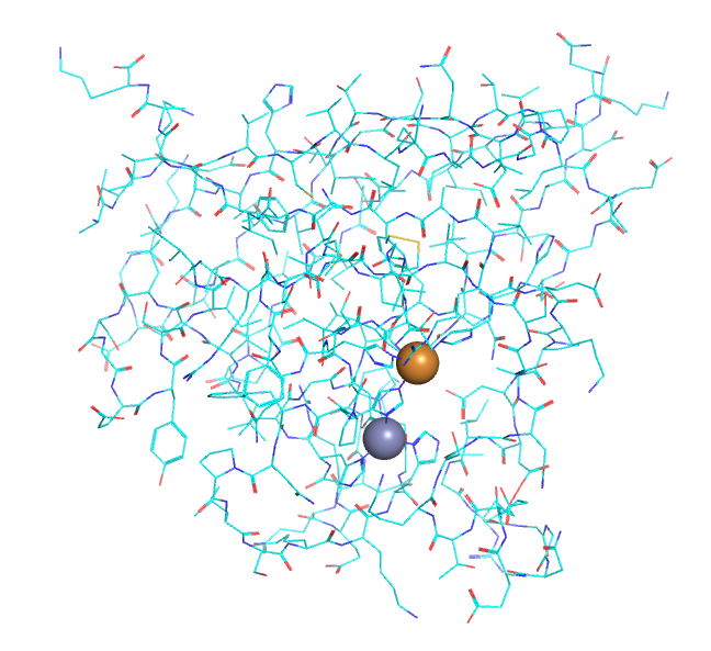
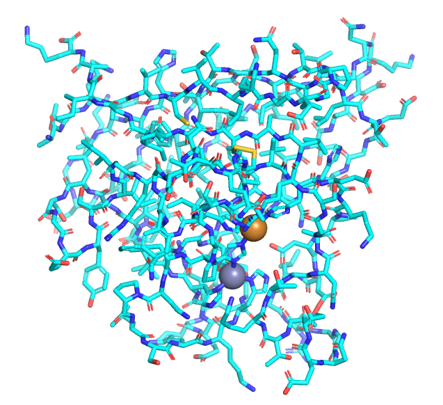
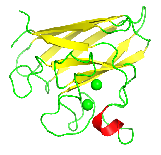
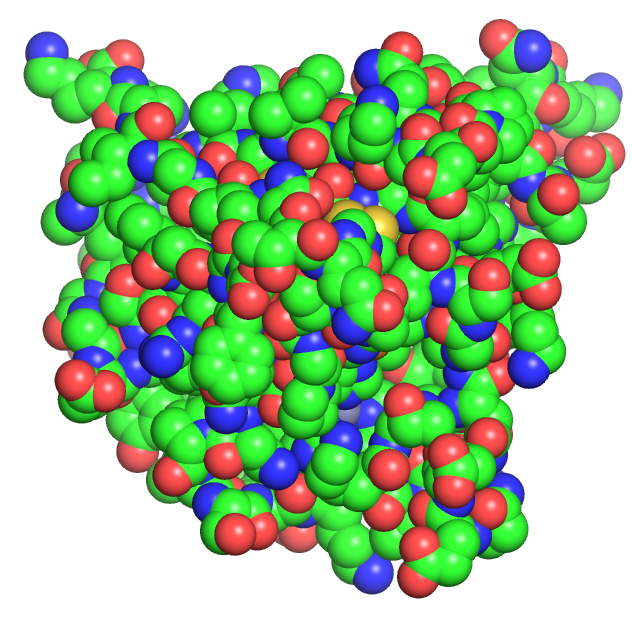
As molecules get larger, line, stick, and ball-and-stick representations become increasingly useless. New ways of visualizing the molecular structure are needed. The importance of multiple renderings to clarify structure/function relationships becomes apparent when you wish to understand protein structure. Various renderings of the protein superoxide dismutase (2sod) are shown in Table \(\PageIndex{2}\) below.

line	stick	cartoon	sphere	surface

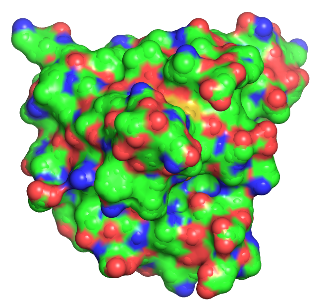Table \(\PageIndex{2}\): Multiple renderings of the protein superoxide dismutase

• The same features and limitations described above for small molecules apply to large ones. It is best to omit most atoms and use mixed renderings within a single display to reveal the biomolecule's crucial structural features. The cartoon representation of superoxide dismutase shows a single tiny alpha helix (red) and many beta strands (yellow). All side chain and backbone atoms have been removed. The green line traces the backbone of amino acids not involved in secondary structure. The Cu and Zn ions are shown as spheres.

Another type of surface rendering, the electrostatic potential surface, is beneficial. Figure \(\PageIndex{3}\) shows the electrostatic potential surface of superoxide dismutase taken from two different angles after simply rotating the protein.

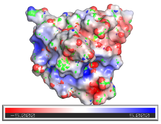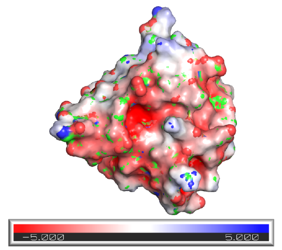Figure \(\PageIndex{3}\): Electrostatic potential surface of superoxidase dismutase from two perspectives

The red represents minimal (most negative) potential. This part of the structure would be enriched in slightly negative Os and Ns, or in wholly negative Os (i.e., with the highest electron density). Blue represents the positive potential centered in regions containing a slight or full positive charge (I, the lowest electron density). This enzyme binds superoxide, O₂^-, a toxic free radical reduction product of dioxygen, \(\ce{O2}\). It catalyzes this reaction:

\[\ce{2 O2^{-} + 2H^{+} → O2 + H2O}. \nonumber \]

The enzyme can effectively scavenge superoxide in its vicinity as the negative superoxide is drawn into the active site with the \(\ce{Cu}\) and \(\ce{Zn}\) atoms by the positive potential surrounding the active site, enhancing the typical diffusion encounter rate of the reactant with the enzyme pocket.

Figure \(\PageIndex{4}\) shows an interactive iCn3D model of the electrostatic potential of superoxidase dismutase (2sod).

Figure \(\PageIndex{4}\): Electrostatic potential of superoxidase dismutase (2sod) (Copyright; author via source).
Click the image for a popup or use this external link: https://structure.ncbi.nlm.nih.gov/i...QQy2hAXehWLBW8

Summary

(Summary written by Claude, Sonnet 4.6, Anthropic)

This short but conceptually important chapter addresses a foundational skill in biochemistry: how to read, interpret, and critically evaluate molecular structure visualizations across scales from small organic molecules to large proteins. It establishes the principle that structure determines function — a theme introduced in introductory chemistry through Lewis structures and molecular geometry — and extends it to the complex, data-derived, computationally rendered structures that dominate modern biochemistry.

Structural data and their limitations deserve explicit attention before any rendering is interpreted. Structures deposited in the Protein Data Bank (PDB) from X-ray crystallography represent electron density maps that are computationally refined into atomic models. Because hydrogen atoms lack sufficient electrons to scatter X-rays effectively, they are absent from essentially all PDB structures; students must mentally add them and infer H-bond donors and acceptors from the positions of nitrogen and oxygen atoms. Crystallographic structures are also inherently static — capturing one conformation from the conformational ensemble that any molecule samples in solution — and may contain modeling errors, including steric clashes, missing atoms, or incorrect atom assignments, although modern refinement protocols minimize these. Cryo-EM structures share similar interpretive considerations and, at lower resolutions, may show only backbone traces rather than side chain detail.

Different rendering styles serve different analytical purposes, and proficiency in biochemistry requires the ability to select the right tool for the question at hand. For small molecules such as oleic acid, line and stick representations clearly show bond connectivity, bond angles, and the cis double bond geometry that distinguishes oleic acid from its trans isomer; ball-and-stick renderings additionally convey relative atomic sizes; spacefill (van der Waals sphere) representations communicate the true steric bulk and shape of the molecule most accurately, and are essential for understanding close-packing, steric hindrance, and solvent accessibility; and surface renderings — calculated from the contact surface swept by a rolling probe atom (typically representing water) over the van der Waals surface — show the molecular shape as encountered by other molecules or solvents. For large proteins such as superoxide dismutase, line and stick renderings become too visually dense to interpret, and cartoon representations become essential: α-helices are shown as ribbons or cylinders, β-strands as flat arrows indicating chain direction, and non-regular regions as tubes tracing the backbone. These cartoons reveal secondary structure content and overall topological organization (e.g., the predominance of β-strands and a single small α-helix in superoxide dismutase) but completely omit side chain information. Mixed renderings — combining cartoon backbone with stick side chains in a region of interest, or displaying a molecular surface with a cartoon visible underneath — provide complementary information that neither mode alone conveys.

Electrostatic potential surfaces are among the most functionally informative renderings available for large molecules. By coloring the molecular surface according to calculated electrostatic potential — with red indicating electron-rich regions (partial or full negative charge) and blue indicating electron-poor regions (partial or full positive charge) — this rendering predicts regions of favorable interaction with charged or polar substrates, inhibitors, or binding partners. For superoxide dismutase, the electrostatic surface reveals a strongly positive channel leading to the active site Cu/Zn center, which electrostatically guides the negatively charged superoxide radical (O₂⁻) toward the active site at rates exceeding simple diffusion — a striking example of how the charge landscape of a protein's surface is shaped by evolution to optimize catalytic efficiency.