19.2: The Genetic Code

The Central Dogma: DNA Encodes RNA; RNA Encodes Protein

To summarize what we know to this point, the cellular process of transcription generates messenger RNA (mRNA), a mobile molecular copy of one or more genes with an alphabet of A, C, G, and uracil (U). Translation of the mRNA template converts nucleotide-based genetic information into a protein product. This flow of genetic information in cells from DNA to mRNA to protein is described by the Central Dogma (Figure \(\PageIndex{1}\)), which states that genes specify the sequence of mRNAs, which in turn specify the sequence of proteins. The decoding of one molecule to another is performed by specific proteins and RNAs. Because the information stored in DNA is so central to cellular function, it makes intuitive sense that the cell would make mRNA copies of this information for protein synthesis, while keeping the DNA itself intact and protected.

It turns out that the central dogma is not always true. We will not discuss the exceptions here, however.

Figure \(\PageIndex{1}\): Instructions on DNA are transcribed onto messenger RNA. Ribosomes are able to read the genetic information inscribed on a strand of messenger RNA and use this information to string amino acids together into a protein.

Amino Acid Structure

Protein sequences consist of 20 commonly occurring amino acids (Figure \(\PageIndex{2}\)); therefore, it can be said that the protein alphabet consists of 20 letters. Different amino acids have different chemistries (such as acidic versus basic, or polar and non-polar) and different structural constraints. Variation in amino acid sequence gives rise to enormous variation in protein structure and function.

Figure \(\PageIndex{2}\): Structures of the 20 amino acids found in proteins are shown. Each amino acid is composed of an amino group (NH₃⁺), a carboxyl group (COO^-), and a side chain (blue). The side chain may be nonpolar, polar, or charged, as well as large or small. It is the variety of amino acid side chains that gives rise to the incredible variation of protein structure and function.

Genetic Code

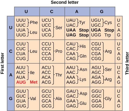
Each amino acid is defined by a three-nucleotide sequence called the triplet codon. The relationship between a nucleotide codon and its corresponding amino acid is called the genetic code. Given the different numbers of “letters” in the mRNA (4 – A, U, C, G) and protein “alphabets” (20 different amino acids) one nucleotide could not correspond to one amino acid. Nucleotide doublets would also not be sufficient to specify every amino acid because there are only 16 possible two-nucleotide combinations (4²). In contrast, there are 64 possible nucleotide triplets (4³), which is far more than the number of amino acids. Scientists theorized that amino acids were encoded by nucleotide triplets and that the genetic code was degenerate. In other words, a given amino acid could be encoded by more than one nucleotide triplet (Figure \(\PageIndex{3}\)). These nucleotide triplets are called codons.

The same codon will always specify the insertion of one specific amino acid. The chart seen in Figure \(\PageIndex{3}\) can be used to translate an mRNA sequence into an amino acid sequence. For example, the codon UUU will always cause the insertion of the amino acid phenylalanine (Phe), while the codon UUA will cause the insertion of leucine (Leu).

Figure \(\PageIndex{3}\): This figure shows the genetic code for translating each nucleotide triplet in mRNA into an amino acid or a termination signal in a nascent protein. (credit: modification of work by NIH)

References

Unless otherwise noted, images on this page are licensed under CC-BY 4.0 by OpenStax.

OpenStax, Biology. OpenStax CNX. January 2, 2017 https://cnx.org/contents/GFy_h8cu@10...fig-ch15_01_05