W2017_Lecture_02_reading

Models and Simplifying Assumptions

Creating Models of Real Things

Life is complicated. To help us understand what we see around us - in both our everyday lives and in science or engineering - we often construct models. A common aphorism states: All models are wrong, but some are useful. That is, no matter how sophisticated, all models are approximations of something real. While they are not the “real thing” (and are thus wrong), models are useful when they allow us to make predictions about real life that we can use. Models come in a variety of forms that include, but are not limited to:

Types of Models

• Physical models- these are 3D objects that we can touch.
• Drawings - these can be on paper or on the computer and either in 2D or virtual 3D. We mostly look at them.
• Mathematical models - these describe something in real life in mathematical terms. We use these to calculate the behavior of the thing or process we want to understand.
• Verbal or written models - these models are communicated in written or spoken language.
• Mental models - these models are constructed in our minds and we use these to create the other types of models and to understand the things around us.

Simplifying Assumptions

Usually, in science and everyday life alike, simple models are preferred over complex ones. Creating simple models of complex real things requires us to make what are known as simplifying assumptions. As their name implies, simplifying assumptions are assumptions that are included in the model to simplify the analysis as much as possible. When a simplified model no longer predicts behavior of the real thing within acceptable bounds, too many simplifying assumptions have been made. When little predictive value is gained from adding more details to a model, it is likely overly complex. Let’s take a look at different types of models from different disciplines and point out their simplifying assumptions.

An example from physics: A block on a frictionless plane

A line drawing that models a block (of any material) sitting on a generic incline plane. In this example some simplifying assumptions are made. For instance, the details of the materials the block and plane are made of are ignored. Often we might also for convenience assume that the plane is frictionless. The simplifying assumptions allow the student to practice thinking about how to balance the forces acting on the block when it is elevated in a gravity field and the surface that it is sitting on is not perpendicular to the gravity vector (mg). This simplifies the math and allows the student to focus on the geometry of the model and how to represent that mathematically. The model, and its simplifying assumptions, might do a reasonably good job of predicting the behavior of an ice cube sliding down an glass incline plane but would likely do a bad job of predicting the behavior of a wet sponge on an incline plane coated with sand paper. The model would be oversimplified for the latter scenario.

Source: Created by Marc T. Facciotti (Own work)

An example from biology: a ribbon diagram of a protein - The transmembrane protein bacteriorhodopsin

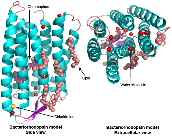
This is a cartoon model of the transmembrane protein bacteriorhodopsin. The protein is represented as a light blue and purple ribbon (the different colors highlight alpha helix and beta sheet, respectively), a chloride ion is represented as a yellow sphere, red spheres represent water molecules, pink balls-and-sticks represent a retinal molecule located on the "inside" of the protein, and orange balls-and-sticks represent other lipid molecules located on the "outside" surface of the protein. The model is displayed in two views. On the left the model is viewed "side on" while on the right it is viewed along its long axis from the extracellular side of the protein (rotated 90 deg out of the page from the view on the left). This model simplifies many of the atomic-level details of the protein. It also fails to represent the dynamics of the protein. The simplifying assumptions mean that the model would not do a good job predicting the time it takes for the protein to do its work or how many protons can be transported across a membrane per second. On the other hand, this model does a very good job of predicting how much space the protein will take up in a cellular membrane, how far into the membrane the retinal sits, or whether certain compounds can reasonably “leak” through the inner channel.

Source: Created by Marc T. Facciotti (own work), University of California, Davis
Derived from PDBID:4FPD

An example from Chemistry: A molecular line model of glucose

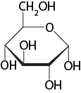
Figure 3: A line drawing of a glucose molecule. By convention, the points where straight lines meet are understood to represent carbon atoms while other atoms are shown explicitly. Given some additional information about the nature of the atoms that are figuratively represented here, this model can be useful for predicting some of the chemical properties of this molecule, including solubility or the potential reactions it might enter into with other molecules. The simplifying assumptions however hide the dynamics of the molecules.

Source: Created by Marc T. Facciotti (Own work)

An example from everyday life: A scale model of a Ferrari

A scale model of a Ferrari. There are many simplifications and most only make this useful for predicting the general shape and relative proportions of the real thing. For instance, this model gives us no predictive power about how well the car drives or how quickly it stops from a speed of 70 km/s.

Source: Created by Marc T. Facciotti (Own work)

Note: Possible discussion

Describe a physical model that you use in everyday life. What does the model simplify from the real thing?

Note: Possible discussion

Describe a drawing that you use in science class to model something real. What does the model simplify from the real thing? What are the advantages and disadvantages of the simplifications?

The spherical cow

The spherical cow is a famous metaphor in physics that make fun of physicists tendencies to create hugely simplified models for very complex things. Numerous jokes are associated with this metaphor and they go something like this:

"Milk production at a dairy farm was low, so the farmer wrote to the local university, asking for help from academia. A multidisciplinary team of professors was assembled, headed by a theoretical physicist, and two weeks of intensive on-site investigation took place. The scholars then returned to the university, notebooks crammed with data, where the task of writing the report was left to the team leader. Shortly thereafter the physicist returned to the farm, saying to the farmer, "I have the solution, but it only works in the case of spherical cows in a vacuum"."
Source: Wikipedia page on Spherical Cow - accessed November 23, 2015.

A cartoon representation of a spherical cow.
Source: https://upload.wikimedia.org/wikiped.../d2/Sphcow.jpg
By Ingrid Kallick (Own work) [GFDL (http://www.gnu.org/copyleft/fdl.html) or CC BY 3.0 (http://creativecommons.org/licenses/by/3.0)], via Wikimedia Commons

The spherical cow is an amusing way to ridicule the process of creating simple models and it is quite likely that you will have your BIS2A instructor invoke the reference to the spherical cow when an overly simplified model of something in biology is being discussed. Be ready for it!

Bounding or Asymptotic Analysis

In BIS2A we use models frequently. Sometimes we also like to imagine or test how well our models actually represent reality and compare that with expectations from what we know to be true for the real life thing. There are many ways to do this depending on how precisely you need to know the behavior of the thing you're trying to model. If you need to know a lot of detail, you create a detailed model. If you're willing to live with less detail, you will create a simpler model. In addition to applying simplifying assumptions, it is often useful to assess your model using a technique we call bounding or asymptotic analysis. The main idea of this technique is to use the model, complete with simplifying assumptions, to understand how the real thing might behave at extreme conditions (e.g. evaluate the model at the minimum and maximum values of a variable). Let’s examine a simple real life example of how this technique works:

Example: Bounding

Problem setup
Imagine that you need to leave Davis, CA and get home to Selma, CA for the weekend. It's 5PM and you told your parents that you'd be home by 6:30. Selma is 200 miles (322 kM) from Davis. You're getting worried that you won't make it home on time. Can you get some estimate of whether it's even possible or if you'll be reheating your dinner in the microwave?

Create Simplified Model and Use of Bounding
You can create a simplified model. In this case you can assume that the road between Davis and Selma is perfectly straight. You also assume that your car has only 2 speeds: 0 mph and 120 mph. These two speeds are the minimum and maximum speeds that you can travel - the bounding values. You can now estimate that even under assumptions of the theoretically "best case" scenario, where you would drive on a perfectly straight road with no obstacles or traffic at maximum speed, you will not make it home on time. At maximum speed you would only cover 180 of the required 200 miles in the 1.5 hours you have.

Interpretation
In this real-life example a simplified model is created. In this case, one very important simplifying assumptions is made: The road is assumed to be straight and free of obstacles or traffic. These assumptions allow you to reasonably assume that you could drive this road at full speed the whole distance. The simplifying assumptions simplified out a lot of what you know is actually there in the real world that would influence the speed you could travel and by extension the time it would take to make the trip. The use of bounding – or calculating the behavior of at the minimum and maximum speeds is a way of making quick predictions about what might happen in the real world.

We will conduct similar analyses in BIS2A.

The importance of knowing key model assumptions

Knowing what simplifying assumptions are made in a model is critical to judging how useful it is for predicting real life and for starting to make a guess about where the model needs improving if it is not sufficiently predictive. In BIS2A you will periodically be asked to create different types of models and to explicitly identify the simplifying assumptions and the impact of those assumptions on the utility and predictive ability of the model. We will also use models together with bounding exercises to try learning something about the potential behavior of a system.

------------------------------------------------------------------------------------------------------------------------------------------------------------

General Approach to Biomolecule Types in Bis2a

Some context and motivation

In BIS2A we are concerned primarily with developing a functional understanding of a biological cell. In the context of a design problem we might say that we want to solve the problem of building a cell. If we break this big task down into smaller problems or alternatively ask what types of things do we need to understand in order to do this, it would be reasonable to conclude that understanding what the cell is made of would be important. That said, it isn't sufficient to appreciate WHAT the cell is made of. We also need to understand the PROPERTIES of the materials that make up the cell. This requires us to dig into a little bit of chemistry - the science of the "stuff" (matter) that makes up the world we know.

This prospect of talking about molecular chemistry and thermodynamics makes some students of biology apprehensive. Hopefully, however, we will show that many of the vast number of biological processes that we care about arise directly from the chemical properties of the "stuff" that makes up life and that developing a functional understanding of some basic chemical concepts can be tremendously useful in thinking about how to solves problems in medicine, energy, and environment by attacking them at their core.

Importance of chemical composition

As a student in BIS2A, you will be asked to classify macromolecule into groups by looking at their chemical composition and based on this composition also infer some of the properties they might have. For example, carbohydrates typically have multiple hydroxyl groups. Hydroxyl groups are polar functional groups capable of forming hydrogen bonds. Therefore, some of the biologically relevant properties of various carbohydrates can be understood at some level by a balance between how they my tend to form hydrogen bonds with water, themselves or other molecules.

Linking structure to function

Each macromolecule plays a specific role in the overall functioning of a cell. The chemical properties and structure of a macromolecule will be directly related to its function. For example, the structure of a phospholipid can be broken down into two groups, a hydrophilic head group and a hydrophobic tail group. Each of these groups plays a role in not only the assembly of the cell membrane but also in the selectivity of substances that can/cannot cross the membrane.

------------------------------------------------------------------------------------------------------------------------------------------------------------

Atoms are the building blocks of molecules found in the universe—air, soil, water, rocks . . . and also the cells of all living organisms. In this model of an organic molecule, the atoms of carbon (black), hydrogen (white), nitrogen (blue), oxygen (red), and sulfur (yellow) are shown in proportional atomic size. The silver rods represent chemical bonds. (credit: modification of work by Christian Guthier)

The Structure of an Atom

An atom is the smallest unit of matter that retains all of the chemical properties of an element. Elements are forms of matter with specific chemical and physical properties that cannot be broken down into smaller substances by ordinary chemical reactions.

The chemistry discussed in BIS2A requires us to use a model for an atom. While there are more sophisticated models, the atomic model used in this course makes the simplifying assumption that the standard atom is composed of three sub-atomic particles, the proton, the neutron, and the electron. Protons and neutrons have a mass of approximately 1 atomic mass unit (a.m.u.). One atomic mass unit is approximately 1.660538921 ×10^-27kg - roughly 1/12 of the mass of a carbon atom (see table below for more precise value). The mass of an electron is 0.000548597 a.m.u. or 9.1 x 10^-31kg. Neutrons and protons reside at the center of the atom in a region call the nucleus while the electrons orbit around the nucleus in zones called orbitals, as illustrated below. The only exception to this description is the hydrogen (H) atom, which is composed of one proton and one electron with no neutrons. An atom is assigned an atomic number based on the number of protons in the nucleus. Neutral carbon (C), for instance has 6 neutrons, 6 protons and 6 electrons. It has an atomic number of 6 and a mass of slightly more than 12 a.m.u.

Protons, Neutrons, and Electrons
	Charge	Mass (a.m.u.)	Mass (kg)	Location
Proton	+1	~1	1.6726x10^-27	nucleus
Neutron	0	~1	1.6749x10^-27	nucleus
Electron	–1	~0	9.1094x10^-31	orbitals

TABLE: Charge, mass, and location of sub-atomic particles

This table reports the charge and location of three subatomic particles - the neutron, proton, and electron. a.m.u. = atomic mass unit (aka. dalton - symbol Da) - this is defined as approximately one twelfth of the mass of a neutral carbon atom or 1.660538921 × 10⁻²⁷ kg. This is roughly the mass of a proton or neutron.

Elements, such as helium, depicted here, are made up of atoms. Atoms are made up of protons and neutrons located within the nucleus and electrons surrounding the nucleus in regions called orbitals. (Note: This figure depicts a Bohr model for an atom - we could use a new open-source figure that depicts a more modern model for orbitals. If anyone finds one please forward it.)
Source:(https://commons.wikimedia.org/wiki/F...um_atom_QM.svg)
By User:Yzmo (Own work) [GFDL (http://www.gnu.org/copyleft/fdl.html) or CC-BY-SA-3.0 (http://creativecommons.org/licenses/by-sa/3.0/)], via Wikimedia Commons

Relative sizes and distribution of elements

The typical atom has a radius of 1-2 angstroms(Å). 1Å = 1 x 10^-10m. The typical nucleus has a radius 1 x 10^-5Å or 10,000 smaller than the radius of the whole atom. By analogy, a typical large exercise ball has a radius of 0.85m. If this were an atom, the nucleus would have a radius about 1/2 to 1/10 of your thinnest hair. All of that extra volume is occupied by the electrons in regions called orbitals. For an ideal atom, orbitals are probabilistically defined regions in space around the nucleus in which an electron can be expected to be found.

For additional basic information on atomic structure click here.
For additional basic information on orbitals here.

Video clips

For a review of atomic structure check out this You-tube video: atomic structure.

The properties of living and non-living materials are determined to a large degree by the composition and organization of their constituent elements. Five elements are common to all living organisms: Oxygen (O), Carbon (C), Hydrogen (H), Phosphorous (P), and Nitrogen (N). Other elements like Sulfur (S), Calcium (Ca), Chloride (Cl), Sodium (Na), Iron (Fe), Cobalt (Co), Magnesium, Potassium (K), and several other trace elements are also necessary for life but are typically found in far less abundance than the "top five" noted above. As a consequence, life's chemistry - and by extension the chemistry of relevance in Bis2A, largely focuses on common arrangements of and reactions between the "top five" core atoms of biology.

A table illustrating the abundance of elements in the human body. A pie chart illustrating the relationships in abundance between the 4 most common elements.
Credit: Data from Wikipedia (http://en.wikipedia.org/wiki/Abundan...mical_elements); chart created by Marc T. Facciotti

The Periodic Table

The different elements are organized and displayed in the periodic table. Devised by Russian chemist Dmitri Mendeleev (1834–1907) in 1869, the table groups elements that, due to some commonalities of their atomic structure, share certain chemical properties. The atomic structure of elements is responsible for their physical properties including whether they exist as gases, solids, or liquids under specific conditions and and their chemical reactivity, a term that refers to their ability to combine and to chemically bond with each other and other elements.

In the periodic table, shown below, the elements are organized and displayed according to their atomic number and are arranged in a series of rows and columns based on shared chemical and physical properties. In addition to providing the atomic number for each element, the periodic table also displays the element’s atomic mass. Looking at carbon, for example, its symbol (C) and name appear, as well as its atomic number of six (in the upper right-hand corner indicating the number of protons in the neutral nucleus) and its atomic mass of 12.11 (sum of the mass of electrons, protons, and neutrons).

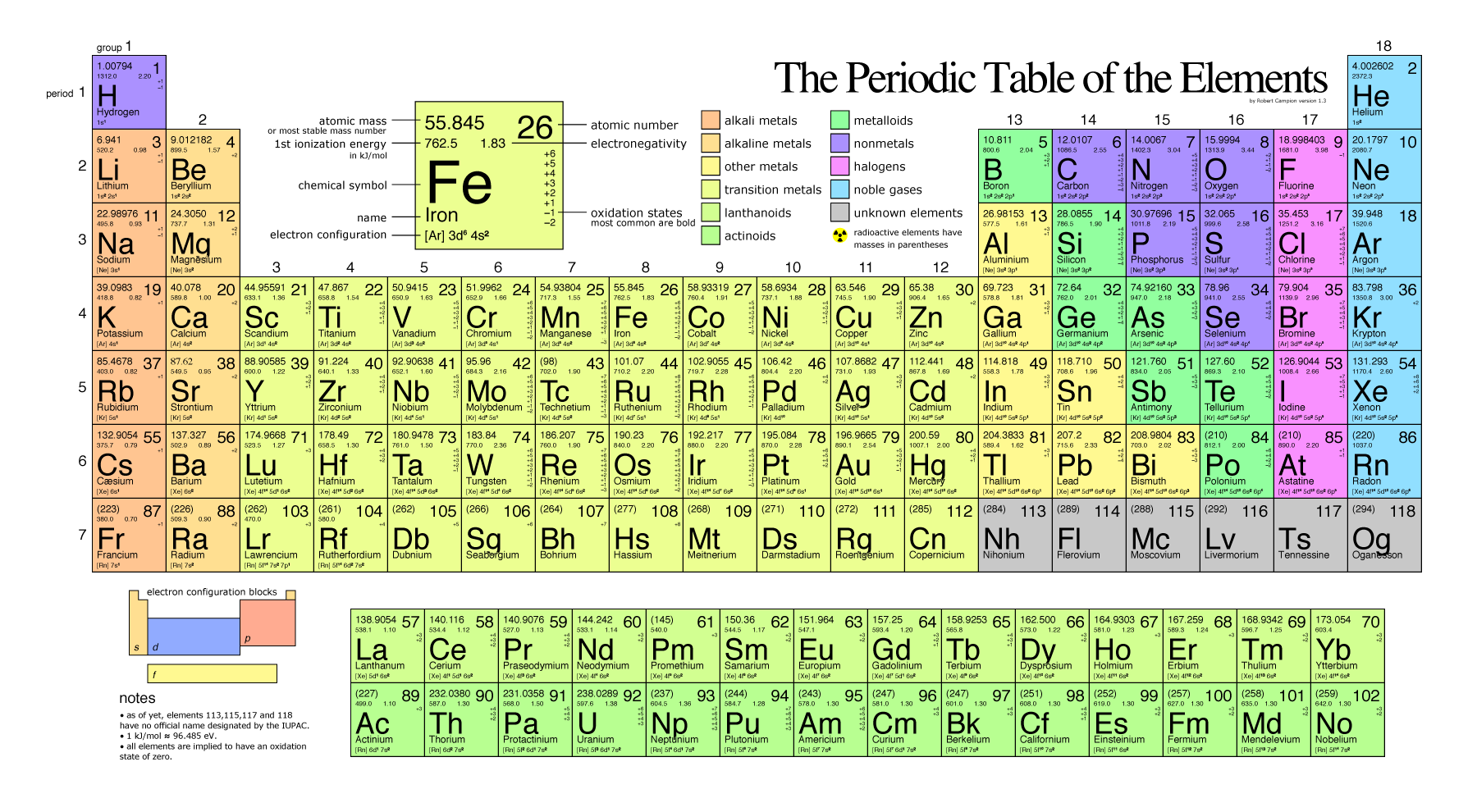
The periodic table shows the atomic mass and atomic number of each element. The atomic number appears above the symbol for the element and the approximate atomic mass appears to the left.
Source: By 2012rc (self-made using inkscape) [Public domain], via Wikimedia Commons Modified by Marc T. Facciotti - 2016

Electronegativity

Molecules are collections of atoms that are associated to one another by bonds. It is reasonable to expect - and the case empirically - that different atoms will exhibit different physical properties, including abilities to interact with other atoms. One such property, the tendency of an atom to attract electrons, is described by the chemical concept and term electronegativity. While several methods for measuring electronegativity have been developed, the one most commonly taught to biologists is the one created by Linus Pauling.

A description of how Pauling electronegativity can be calculated is beyond the scope of Bis2a. What is important to know, however, is that electronegativity values have been experimentally and/or theoretically determined for nearly all elements in the periodic table. The values are unitless and are reported relative to the standard reference, hydrogen, whose electronegativity is 2.20. The larger the electronegativity value the greater tendency an atom has to attract electrons. Using this scale the electronegativity of different atoms can be quantitatively compared. For instance, by using Table 1 below you could report that oxygen atoms are more electronegative than phosphorous atoms.

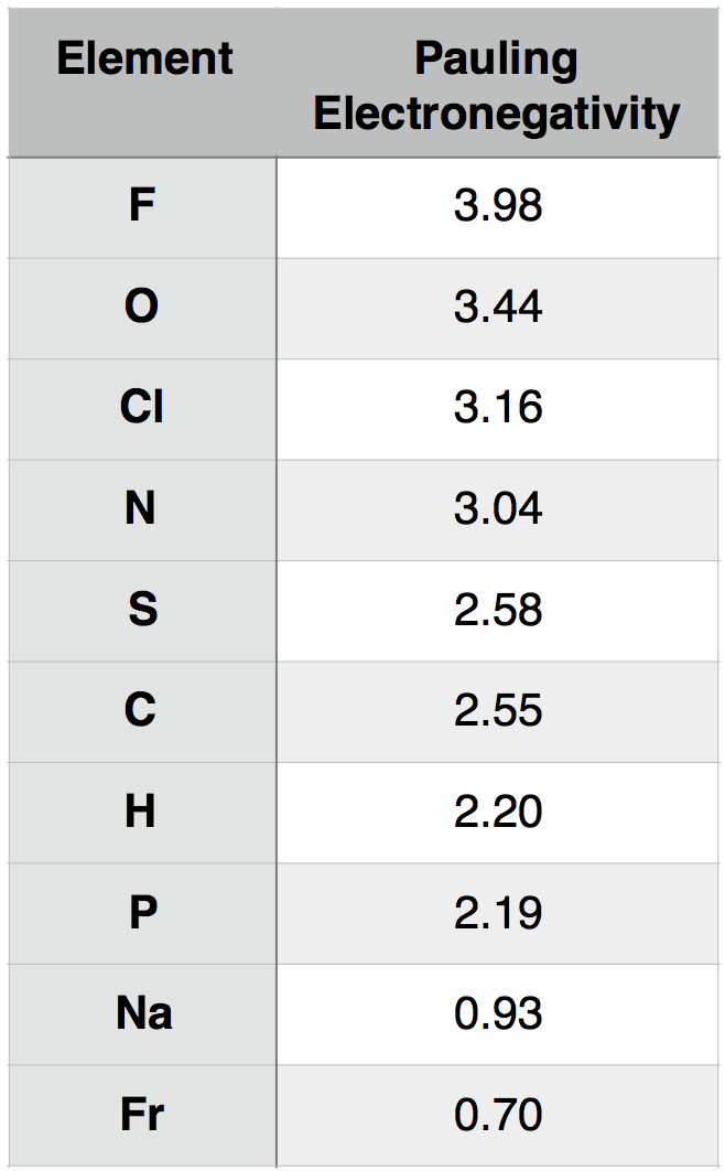
Pauling electronegativity values for select elements of relevance to Bis2A and elements at the two extreme (highest and lowest) of the electronegativity scale.

Attribution: Marc T. Facciotti (original work)

The utility of the Pauling electronegativity scale in Bis2a is to provide a chemical basis for explaining they types of bonds that form between the commonly occurring elements in biological systems and to explain some of the key interactions we observe routinely. We develop our understanding electronegativity-based arguments about bonds and molecular interactions by comparing the electronegativities between two atoms. Recall, the larger the electronegativity, the stronger the "pull" an atom exerts on nearby electrons.

We can consider for example the common interaction between oxygen(O)and hydrogen(H). Let us assume that O and H are interacting (forming a bond) and write that interaction as O-H, where the dash between the letters represents the interaction between the two atoms. To understand this interaction better we can compare the relative electronegativity of each atom. Examining the table above we see that O has an electronegativity of 3.44 and H has an electronegativity of 2.20.

Based on the concept of electronegativity as we now understand it we can surmise that the oxygen (O) atom will tend to "pull" the electrons away from the hydrogen (H) when they are interacting. This will give rise to a slight but significant negative charge around the O atom (due to the higher tendency of the electrons to be associated with the O atom). This also results in a slight positive charge around the H atom (due to the decrease in the probability of finding an electron nearby). Since the electrons are not distributed evenly between the two atoms AND by consequence the electric charge is also not evenly distributed we call this interaction or bond polar. There are in effect two poles; the negative pole near the oxygen and the positive pole near the hydrogen.

To extend the utility of this concept we can now ask how an interaction between oxygen (O) and hydrogen (H) differs from an interaction between sulfur (S) and hydrogen (H). That is how does O-H differ from S-H? If we examine the table above we see that the difference in electronegativity O and H is 1.24 (3.44 - 2.20 = 1.24) and that the difference in electronegativity between S and H is 0.38 (2.58 – 2.20 = 0.38). We can therefore conclude that an O-H bond is more polar than an S-H bond. We will discuss the consequences of these differences in subsequent chapters.

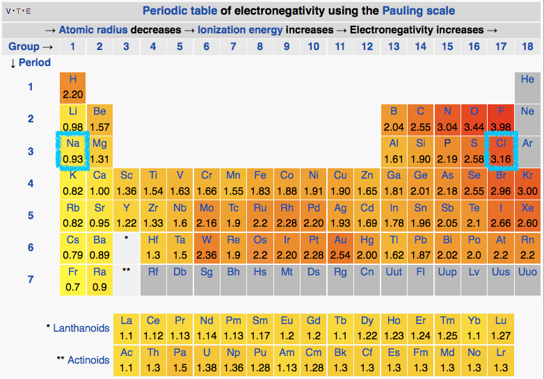
The periodic table with the electronegativities of each atom listed.
Attribution: By DMacks (https://en.wikipedia.org/wiki/Electronegativity) [CC BY-SA 3.0 (http://creativecommons.org/licenses/by-sa/3.0)], via Wikimedia Commons

An examination of the periodic table of the elements (Figure above) illustrates that electronegativity is related to some of the physical properties used to organize the elements into the table. Certain trends are apparent. For instance, those atoms with the largest electronegativity tend to reside in the upper right hand corner of the periodic table, such as Fluorine (F), Oxygen (O) and Chlorine (Cl), while elements with the smallest electronegativity tend to be found at the other end of the table, in the lower left, such as Francium (Fr), Cesium (Cs) and Radium (Ra).

More information on electronegativity can be found in the LibreTexts

The main use of the concept of electronegativity in Bis2a will therefore be to provide a conceptual grounding for discussing the different types of chemical bonds that occur between atoms in Nature. We will focus primarily on three types of bonds: Ionic Bonds, Covalent Bonds and Hydrogen Bonds.

Bond Types

In Bis2a we focus primarily on three different bond types: ionic bonds, covalent bonds, and hydrogen bonds. We expect students to be able to recognize each different bond type in molecular models. In addition, for commonly seen bonds in biology, we expect student to provide an chemical explanation, rooted in ideas like electronegativity, for how these bonds contribute to the chemistry of biological molecules.

Ionic Bonds

Ionic bonds are electrostatic interactions formed between ions of opposite charges. For instance, most of us appreciate that sodium chloride (NaCl)positively charged sodium ions and negatively charged chloride ions associate via electrostatic (+ attracts -) interactions to make crystals of sodium chloride, or table salt, creating a crystalline molecule with zero net charge. These origins of these interactions may arise from the association of neutral atoms whose difference in electronegativities is sufficiently high. Take the example above. If we imagine that a neutral sodium atom and a neutral chlorine atom approached one another it is possible that at close distances, due to the relatively large difference in electronegative between the two atoms that an electron from the neutral sodium atom was transferred to the neutral chloride atom, resulting in a negatively charged chloride ion and a positively charged sodium ions. These ions can now interact via an ionic bond.

The formation of an ionic bond between sodium and chloride is depicted. In panel A, a sufficient difference in electronegativity between sodium and chloride induce a transfer of electron from the sodium to the chloride forming two ions illustrated in panel b. In panel c the two ions associate via an electrostatic interaction.

Attribution: By BruceBlaus (Own work) [CC BY-SA 4.0 (http://creativecommons.org/licenses/by-sa/4.0)], via Wikimedia Commons

This movement of electrons from one atom to another is referred to as electron transfer. In the example above, when sodium loses an electron, it now has 11 protons, 11 neutrons, and 10 electrons, leaving it with an overall charge of +1 (summing charges: 11 protons at +1 charge each and 10 electrons at -1 charge each = +1). Once charged the the sodium atom is referred to as a sodium ion. Likewise, based on its electronegativity, a neutral chlorine (Cl) atom tends to gain an electron to create an ion with 17 protons, 17 neutrons, and 18 electrons, giving it a net negative (–1) charge. It is now referred to as a chloride ion.

We can interpret the electron transfer above using the concept of electronegativity. Begin by comparing the electronegativities of sodium and chlorine by examining the periodic table of elements below. We see that chlorine is located on the upper right hand corner of the table while sodium is on the upper left. Comparing the electronegativity values of chlorine and sodium directly we see that the chlorine atom is more electronegative than its sodium counterpart. The difference in the electronegativity of chlorine (3.16) and sodium (0.93) is 2.23 (using the scale in the table below). Given that we know an electron transfer will take place between these two element, we can conclude that differences in electronegativities of of ~2.2 are large enough to cause an electron transfer between two atoms and that interactions between such elements are likely through ionic bonds.

The periodic table of the elements listing electronegativity values for each element. The elements sodium and chlorine are boxed with a teal boundary. Attribution: By DMacks (https://en.wikipedia.org/wiki/Electronegativity) [CC BY-SA 3.0 (http://creativecommons.org/licenses/by-sa/3.0)], via Wikimedia Commons - Modified by Marc T. Facciotti

Note:

Possible Discussion: The atoms in a 5 in. x 5 in. brick of table salt (NaCl) sitting on your kitchen counter are held together almost entirely by ionic bonds. Based on that observation how would you characterize the strength of ionic bonds?

Now consider that same brick of table salt after having been thrown into an average backyard swimming pool. After a couple of hours the brick would be completely dissolved and the sodium and chloride ions would be uniformly distributed throughout the pool. What might you conclude about the strength of ionic bonds from this observation?

Propose a reason why the ionic bonds in air might be behaving differently than those in water? What is the significance of this to biology?

For additional information:

Check out the link from the Khan academy on ionic bonds.

Covalent Bonds

We can also invoke the concept of electronegativity to help describe the interactions between atoms of similar electronegativity, differences that are smaller than required to form an ionic bond. These types of associations often result in a bond called a covalent bond. In these bonds, electrons are shared between two atoms - in contrast to an ionic interaction in which electrons remain on each atom of an ion or are transferred between species of highly different electronegativities.

We start by exploring the covalent bond by looking at an example where the difference in electronegativity is zero. Consider a very common interaction in biology, the interaction between two carbon atoms. In this case each atom has the same electronegativity, 2.55; the difference in electronegativity is therefore zero. If we build our mental model of this interaction using the concept of electronegativity we realize that each atom in the carbon carbon pair has the same tendency to "pull" electrons to it. In this case when a bond is formed neither of the two atoms will tend to "pull" (a good anthropomorphism) electrons from the other, they will "share" (another anthropomorphism) the electrons equally, instead.

A side:

Bounding Example: The two examples above (1) the interaction of sodium and chlorine and (2) the interaction between two carbon atoms is an example of framing a discussion by bounding or asymptotic analysis (see earlier reading). We examined what happens to a physical system when considering two extremes. In this case the extremes were in electronegativity differences between interacting atoms. The interaction of sodium and chlorine illustrated what happens when two atoms have a large difference in electronegativities and the carbon carbon example illustrated what happens when that difference is zero. Once we have those mental goal posts describing what happens at the extremes it is then easier to imagine what might happen in between - in this case what happens at differences of electronegativity that are in between 0 and 2.2. We do that next.

When the sharing of electrons between two covalently bonded atoms if nearly equal we call these bonds non-polar covalent bonds. If by contrast, the sharing of electrons is not equal between the two atoms (likely due to a difference in electronegativities between atoms) we call these bonds polar covalent bonds.

In a polar covalent bonds, the electrons are unequally shared by the atoms and are attracted to one nucleus more than to the other. Because of the unequal distribution of electrons between atoms in a polar covalent bond, a slightly positive (indicated δ+) or slightly negative (indicated δ–) charge develops on each pole of the bond. This slightly positive (δ+) charge will develop on the less electronegative atom as electrons get pulled more towards the slightly more electronegative atom. A slight negative charge (indicated δ–) charge will develop on the more electronegative atom. Since there are two poles (the positive and negative poles) the bond is said to possess a dipole.

Examples of Nonpolar Covalent and Polar Covalent Bonds in Biologically Relevant Molecules

Nonpolar covalent bonds

Molecular Oxygen

Molecular oxygen (O₂) is an association between two atoms of oxygen. Since the two atoms share the same electronegativity the bonds in molecular oxygen non-polar covalent.

Methane

Another example of a nonpolar covalent bond is the C-H bond found in gas methane (CH₄). Unlike the case of molecular oxygen where the two bonded atoms share the same electronegativity, carbon and hydrogen do not have the same electronegativity; C = 2.55 and H = 2.20 - the difference in electronegativity is 0.35.

Molecular line drawings of molecular oxygen, methane and carbon dioxide.

Attribution: Marc T. Facciotti (own work)

Some of you may now be confused. If there is a difference in electronegativity between the two atoms is the bond not by definition polar? The answer is both yes and no and depends on the definition of polar that the speaker/writer is using. Since this is an example of how shortcuts in the use of specific vocabulary can sometimes lead to confusion we take a moment to discuss this here. See the mock exchange between student and instructor below for clarification:

1. Instructor: "In biology we often that the C-H bond is nonpolar."

2. Student: "But there is an electronegativity difference between C and H and therefore it would appear that C should have a little bit more tendency to attract electrons. This difference should create a small negative charge around the carbon and a small positive charge around the hydrogen."

3. Student: "Since there is a differential distribution of charge across the bond it would seem that, by definition, this should be considered a polar bond."

4. Instructor: "In fact, the bond does have some small polar character." 5. Student: "So, then it's polar? I'm confused."

6. Instructor: "It has some small amount of polar character but it turns out that for most of the common chemistry that we will encounter that this small amount of polar character is insufficient to lead to "interesting" chemistry. So, the while the bond is strictly slightly polar, from a practical standpoint it is effectively nonpolar. We therefore call it non polar."

7. Student: "That's needlessly confusing, how am I supposed to know when you mean strictly 100% nonpolar, slightly polar, or functionally polar when you use the same word to describe two of those three things?"

8. Instructor: "Yup, it sucks. The fix is that I need to be as clear as I can when I talk with you about "polarity" about how I am using the term. I also need to inform you that you will find this (and other) shortcut used when you go out into the field and encourage you to start learning to recognize what is intended by the context of the conversation.

An real-world analogy of this same problem might be the use of the word "newspaper". It can be used in a sentence to refer to the company that publishes some news OR it can refer to the actual item that the company produces. In this case the disambiguation is easily made by native English speakers who can read meaning from the context; new learners may be more confused. Don't worry, as you see more examples of technical word use in science you'll learn to read the meaning from context too."

A side:

How large should the difference in electronegativity be in order to create a bond that has sufficient polar character that we decide to call it polar in biology? Of course, the exact value depends on a number of factors but as a loose rule of thumb we sometimes use a difference of 0.4 as a guesstimate.

This extra information is purely for your information. You will not be asked to assign polarity based on this criteria in Bis2a. You should however appreciate the concept of how polarity can be determined by using the concept of electronegativity, the functional consequences of polarity (more on this in other sections), and the nuance associated with these terms (the discussion above).

Polar covalent bonds

The polar covalent bond can be illustrated by examining the association between O and H in water (H2O). Oxygen has an electronegativity of 3.44 while hydrogen has an electronegativity of 2.20. The difference of electronegativity is 1.24. It turns out that this size of electronegativity difference is large enough that the dipole across the bond contributes to chemical phenomena that we will be interested in.

This is also a good point to mention another common source of student confusion regarding the use of the term polar. Water has polar bonds. This statement refers specifically to the individual O-H bonds. Each of these bonds has a dipole. However, students will also hear that water is a polar molecule. This is also true. This latter statement is referring to the fact that the sum of the two bond dipoles creates a dipole across the whole molecule. A molecule may be nonpolar but still have some polar bonds.

A water molecule has two polar O-H bonds. Since the distribution of charge in the molecule is asymmetric (due to the number and relative orientation of the bond dipoles) the molecule is also polar. The element name and electronegativities are reported in the respective sphere.

Attribution: Marc T. Facciotti (own work)

For additional information: View this short video to see an animation of ionic and covalent bonding.

The continuum of bonds between covalent and ionic

The discussion of bond types above highlights that in nature you will see bonds on a continuum from completely non-polar covalent to purely ionic depending on the atoms that are interacting. As you proceed through your studies you will further discover that in larger, multi-atom molecules, the localization of electrons around an atom is also influenced by multiple factors. For instance, other atoms that are also bonded nearby will exert an influence on the electron distribution around a nucleus in a way that is not easily accounted for by invoking simple arguments of pairwise comparisons of electronegativity. Local electrostatic fields produced by other non-bonded atoms may also have an influence. Recall, reality is always more complicated than our models. However, if the models allow us to reason and predict with "good enough" precision or to understand some key underlying concepts that can be extend later they are quite useful.

Key Bonds in Bis2a

Fortunately, in Bis2A we are largely concerned by the chemical behavior of and bonds between atoms in biomolecules. Since biological systems are composed by a relatively small number of common elements (e.g. C, H, N, O, P, S) and some key ions (e.g. Na+, Cl-, Ca2+, K+, etc.). Start recognizing commonly occurring bonds and the chemical properties that we often see them showing. Some common bonds include C-C, C-O, C-H, N-H, C=O, C-N, P-O, O-H, S-H, and some variants. These will be discussed further in the context of functional groups. The task is not as daunting as it seems.