4.2.4: Population Demography

Unit 4.2.4 - Population Demography

• Please read and watch the following Learning Resources
• Reading the material for understanding, and taking notes during videos, will take approximately 1 hour.
• Optional Activities are embedded.
• Bolded terms are located at the end of the unit in the Glossary. There is also a Unit Summary at the end of the Unit.
• To navigate to Unit 4.2.5, use the Contents menu at the top of the page OR the right arrow on the side of the page.
  • If on a mobile device, use the Contents menu at the top of the page OR the links at the bottom of the page.

Learning Objectives

• Describe how ecologists measure population size and density
• Describe three different patterns of population distribution
• Use life tables to estimate mortality rates
• Describe the three types of survivorship curves and relate them to specific populations

Introduction

Populations are dynamic entities. Populations consist of a species living within a specific area, and populations fluctuate based on a number of factors: seasonal and yearly changes in the environment, natural disasters such as forest fires and volcanic eruptions, and competition for resources between and within species. The statistical study of population dynamics, demography, uses a series of mathematical tools to investigate how populations respond to changes in their biotic and abiotic environments. Many of these tools were originally designed to study human populations. For example, life tables, which identify the life expectancies of individuals within a population and are discussed in more detail in a later section, were initially developed by life insurance companies to set insurance rates. In fact, while the term “demographics” is commonly used when discussing humans, all living populations can be studied using this approach.

Population Size and Density

The study of any population usually begins by determining how many individuals of a particular species exist, and how closely associated they are with each other. Within a particular habitat, a population can be characterized by its population size (N), the total number of individuals, and its population density, the number of individuals within a specific area or volume. Population size and density are the two main characteristics used to describe and understand populations. For example, populations with more individuals may be more stable than smaller populations based on their genetic variability, and thus their potential to adapt to the environment. Alternatively, a member of a population with low population density (more spread out in the habitat), might have more difficulty finding a mate to reproduce compared to a population of higher density. As is shown in Figure \(\PageIndex{1}\), smaller organisms tend to be more densely distributed than larger organisms.

Figure \(\PageIndex{1}\): Australian mammals show a typical inverse relationship between population density and body size.

Optional Activity \(\PageIndex{1}\)

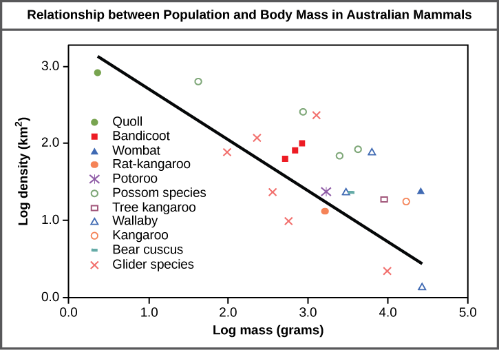
Figure \(\PageIndex{1}\): As this graph shows, population density typically decreases with increasing body size. Why do you think this is the case?

Answer

Smaller animals require less food and other resources, so the environment can support more of them.

Population Research Methods

The most accurate way to determine population size is to simply count all of the individuals within the habitat. However, this method is often not logistically or economically feasible, especially when studying large habitats. Thus, scientists usually study populations by sampling a representative portion of each habitat and using this data to make inferences about the habitat as a whole. A variety of methods can be used to sample populations to determine their size and density.

Video

Ecologists are interested in the distribution of organisms within habitats, and use transects, quadrants, and other sampling methods to collect quantitative data, as you will see in this 5-minute video.
Question after watching: What type of technique would be used for mobile organisms?

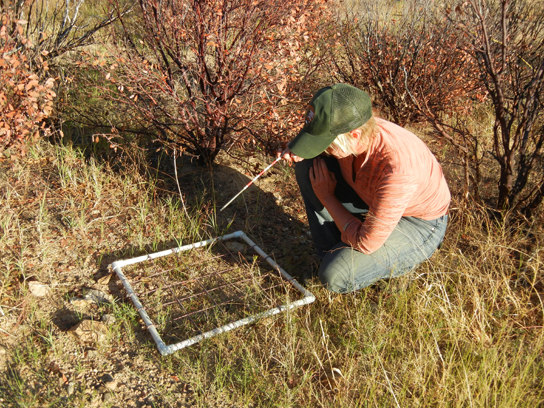
Quadrat Sampling

For immobile organisms such as plants, or for very small and slow-moving organisms, a quadrat may be used. A quadrat is a way of marking off square areas within a habitat, either by staking out an area with sticks and string, or by the use of a wood, plastic, or metal square placed on the ground (Figure \(\PageIndex{2}\)). After setting the quadrats, researchers then count the number of individuals that lie within their boundaries. Multiple quadrat samples are performed throughout the habitat at several random locations. All of this data can then be used to estimate the population size and population density within the entire habitat. The number and size of quadrat samples depends on the type of organisms under study and other factors, including the density of the organism. For example, if sampling daffodils, a 1 m² quadrat might be used whereas with giant redwoods, which are larger and live much further apart from each other, a larger quadrat of 100 m² might be employed. This ensures that enough individuals of the species are counted to get an accurate sample that correlates with the habitat, including areas not sampled.

Figure \(\PageIndex{2}\): A scientist uses a quadrat to measure population size and density. (credit: NPS Sonoran Desert Network)

Distance Sampling Methods

Other techniques for sampling populations to estimate density or abundance are distance sampling methods (Figure \(\PageIndex{3}\)). The main methods are based on line transects or point transects. Distance-based methods are frequently used for animals with observers making their observations while walking, riding in trucks, or in low-flying aircraft. They can also be used for tasks such as surveying for very rare trees or plants.

In this method of sampling, the data collected are the distances of the objects being surveyed from these randomly placed lines or points, and the objective is to estimate the average density of the objects within a region. When using line transects, the observer randomly places a straight line or follows some pre-planned route through the habitat of the population of interest, then walks the line or route. Whenever the researcher observes an object of interest (e.g., an animal of the type being surveyed), they record the observation, the distance from their current position to the object (r), as well as the angle of the detection to the transect line (θ). The distance of the object to the transect can then be calculated using trigonometry as x = r * sin(θ). These distances x are the detection distances that will be analyzed in further modeling aspects of the population (e.g., population distribution in space).

Figure \(\PageIndex{3}\): Basic distance sampling survey approach using line transects. A field observer detects an object and records distance r and angle θ to the transect line. This allows the calculation of object distance to the transect (x). All x from the survey are used to model how detectability decreases with distance from the transect, which allows estimation of total population density in the surveyed area. (Elmidae; CC-BY-4.0)

Mark and Recapture

For mobile organisms, such as mammals, birds, or fish, a technique called mark and recapture is often used. This method involves marking a sample of captured animals in some way (such as tags, bands, paint, or other body markings), and then releasing them back into the environment to allow them to mix with the rest of the population; later, a new sample is collected, including some individuals that are marked (recaptured) and some individuals that are unmarked (Figure \(\PageIndex{4}\)).

Figure \(\PageIndex{4}\): Mark and recapture is used to measure the population size of mobile animals such as (a) bighorn sheep, (b) the California condor, and (c) salmon. (credit a: modification of work by Neal Herbert, NPS; credit b: modification of work by Pacific Southwest Region USFWS; credit c: modification of work by Ingrid Taylar)

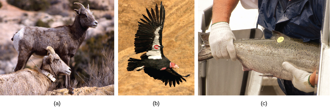
Using the ratio of marked and unmarked individuals, scientists determine how many individuals are in the sample.

To begin, the ratio of the proportions looks like this \[\frac{\text{number marked first catch} {\text{total population}} = \[\frac{\text{number marked second catch} {\text{total caught in second sample}}].

We can rearrange the ratios to solve for an unknown, in this case the total population.

From this, calculations are used to estimate the total population size. This method assumes that the larger the population, the lower the percentage of tagged organisms that will be recaptured since they will have mixed with more untagged individuals.

For example, we will start with 80 deer that are captured, tagged, and released into the forest.

Later, 100 deer are captured and 20 of them are already marked. From this, we can determine the population size (N) using the following equation:

\[\frac{\text{number marked first catch} * \text{total number of second catch}} {\text{number marked second catch}} = N \nonumber\]

Using our example above, 80 would be the number marked first catch, 100 would be the total number of second catch, and 20 would be the number of them already marked.

The calculation of this formula leads to the number 400.

\[\frac{(80*100)} {20} = 400 \nonumber\]

Therefore, there are an estimated 400 total individuals in the original population.

There are some limitations to the mark and recapture method. Some animals from the first catch may learn to avoid capture in the second round, thus inflating population estimates. Alternatively, animals may preferentially be retrapped (especially if a food reward is offered), resulting in an underestimate of population size. Also, some species may be harmed by the marking technique, reducing their survival. A variety of other techniques have been developed, including the electronic tracking of animals tagged with radio transmitters and the use of data from commercial fishing and trapping operations to estimate the size and health of populations and communities.

Camera Traps

Recently, great progress in estimating animal density has been made using camera traps (Figure \(\PageIndex{5}\)). These are especially useful for studying rare and nocturnal animals, such as predators. For example, lions (Panthera leo) are considered vulnerable to extinction and are most threatened in West Africa, where they are restricted to a few small national parks. In western-most West Africa lions occur only in Niokolo-Koba National Park in south-eastern Senegal. Mamadou Kane used camera traps to estimate the density of lions in Niokolo-Koba. While the entire park is 9130 km², Kane sampled an area of approximately 285.4 square kilometers within the highest quality lion habitat of the park. Kane estimated that there are about 3 lions per 100 square kilometers in this high-quality habitat (100 square kilometers is an area 10 km by 10 km). Three lions per 100 km² equals 0.03 per km². We can therefore estimate the total abundance in the study area as 0.03*285.4 = 8.6 lions.

Figure \(\PageIndex{5}\): A camera trap, for taking pictures of game on trails. This model is for hunting. Motion detector on top, lens in the middle, flash on the bottom, with a little LCD for showing how many pictures taken/left on the left. By ​​Hustvedt CC BY-SA 3.0

British Columbia Connection

Many camera traps have been distributed throughout BC to collect data on everything from animal abundance to phenology.

You can view some of these camera trap projects online:

• Parks Canada: https://www.pc.gc.ca/en/nature/science/controle-monitoring/cameras
• Wildlife Cameras for Adaptive Management: https://wildcams.ca/projects/

Optional Activity \(\PageIndex{2}\)

Which of the following methods will tell an ecologist about both the size and density of a population?

1. mark and recapture
2. line transect
3. quadrat
4. camera trap

Answer

c. quadrat sampling

Demography

While population size and density describe a population at one particular point in time, scientists must use demography to study the dynamics of a population. Demography is the statistical study of population changes over time: birth rates, death rates, and life expectancies. Each of these measures, especially birth rates, may be affected by the population characteristics described above. For example, a large population size results in a higher birth rate because more potentially reproductive individuals are present. In contrast, a large population size can also result in a higher death rate because of competition, disease, and the accumulation of waste. Similarly, a higher population density or a clumped dispersion pattern results in more potential reproductive encounters between individuals, which can increase the birth rate. Lastly, a female-biased sex ratio (the ratio of males to females) or age structure (the proportion of population members at specific age ranges) composed of many individuals of reproductive age can increase birth rates.

In addition, the demographic characteristics of a population can influence how the population grows or declines over time. If birth and death rates are equal, the population remains stable. However, the population size will increase if birth rates exceed death rates; the population will decrease if birth rates are less than death rates. Life expectancy is another important factor; the length of time individuals remain in the population impacts local resources, reproduction, and the overall health of the population. These demographic characteristics are often displayed in the form of a life table.

Life Tables

Life tables provide important information about the life history of an organism. Life tables divide the population into age groups and often sexes, and show how long a member of that group is likely to live. They are modeled after actuarial tables used by the insurance industry for estimating human life expectancy. Life tables may include the probability of individuals dying before their next birthday (i.e., their mortality rate), the percentage of surviving individuals dying at a particular age interval, and their life expectancy at each interval.

An example of a life table is shown in Table \(\PageIndex{1}\) from a study of Dall mountain sheep, a species native to northwestern North America. Notice that the population is divided into age intervals (column A). The mortality rate (per 1,000), shown in column D, is based on the number of individuals dying during the age interval (column B) divided by the number of individuals surviving at the beginning of the interval (Column C), multiplied by 1,000.

\[\text{mortality rate} = \frac{\text{number of individuals dying}} {\text{number of individuals surviving}} * 1,000 \nonumber\]

For example, between ages three and four, 12 individuals die out of the 776 that were remaining from the original 1,000 sheep. This number is then multiplied by 1,000 to get the mortality rate per thousand.

\[\text{mortality rate} = \frac{12} {776} * 1,000 \approx 15.5 \nonumber\]

As can be seen from the mortality rate data (column D), a high death rate occurred when the sheep were between 6 and 12 months old, and then increased even more from 8 to 12 years old, after which there were few survivors. The data indicate that if a sheep in this population were to survive to age one, it could be expected to live another 7.7 years on average, as shown by the life expectancy numbers in the last column.

Table \(\PageIndex{1}\): Life Table of Dall Mountain Sheep¹

Age interval (years)	Number dying in age interval out of 1,000 born	Number surviving at beginning of age interval out of 1,000 born	Mortality rate per 1,000 alive at beginning of age interval	Life expectancy or mean lifetime remaining to those attaining age interval
Column A	Column B	Column C	Column D	Column E
0-0.5	54	1000	54.0	7.06
0.5-1	145	946	153.3	--
1-2	12	801	15.0	7.7
2-3	13	789	16.5	6.8
3-4	12	776	15.5	5.9
4-5	30	764	39.3	5.0
5-6	46	734	62.7	4.2
6-7	48	688	69.8	3.4
7-8	69	640	107.8	2.6
8-9	132	571	231.2	1.9
9-10	187	439	426.0	1.3
10-11	156	252	619.0	0.9
11-12	90	96	937.5	0.6
12-13	3	6	500.0	1.2
13-14	3	3	1000	0.7

Survivorship Curves

Another tool used by population ecologists is a survivorship curve, which is a graph of the number of individuals surviving at each age interval plotted versus time (usually with data compiled from a life table). These curves allow us to compare the life histories of different populations (Figure \(\PageIndex{6}\)). Humans and most primates exhibit a Type I survivorship curve because a high percentage of offspring survive their early and middle years—death occurs predominantly in older individuals. These types of species usually have small numbers of offspring at one time, and they give a high amount of parental care to them to ensure their survival. Birds are an example of an intermediate or Type II survivorship curve because birds die more or less equally at each age interval. These organisms also may have relatively few offspring and provide significant parental care. Trees, marine invertebrates, and most fishes exhibit a Type III survivorship curve because very few of these organisms survive their younger years; however, those that make it to an old age are more likely to survive for a relatively long period of time. Organisms in this category usually have a very large number of offspring, but once they are born, little parental care is provided. Thus these offspring are “on their own” and vulnerable to predation, but their sheer numbers assure the survival of enough individuals to perpetuate the species.

Figure \(\PageIndex{6}\): Survivorship curves show the distribution of individuals in a population according to age. Humans and most mammals have a Type I survivorship curve because death primarily occurs in the older years. Birds have a Type II survivorship curve, as death at any age is equally probable. Trees have a Type III survivorship curve because very few survive the younger years, but after a certain age, individuals are much more likely to survive.

Optional Activity \(\PageIndex{3}\)

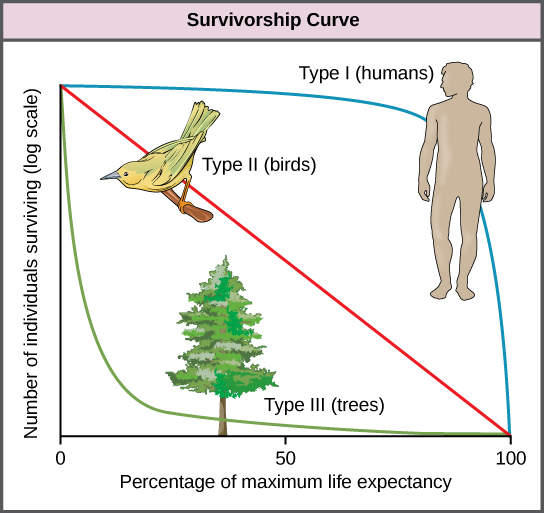
Different species have different survival curves. A Type III survival curve would most likely be observed for _____.

1. whales
2. seals
3. salmon
4. polar bears

Answer

c. salmon