
19.2: Quantifying Food Webs
- Page ID
- 84668
\( \newcommand{\vecs}[1]{\overset { \scriptstyle \rightharpoonup} {\mathbf{#1}} } \)
\( \newcommand{\vecd}[1]{\overset{-\!-\!\rightharpoonup}{\vphantom{a}\smash {#1}}} \)
\( \newcommand{\dsum}{\displaystyle\sum\limits} \)
\( \newcommand{\dint}{\displaystyle\int\limits} \)
\( \newcommand{\dlim}{\displaystyle\lim\limits} \)
\( \newcommand{\id}{\mathrm{id}}\) \( \newcommand{\Span}{\mathrm{span}}\)
( \newcommand{\kernel}{\mathrm{null}\,}\) \( \newcommand{\range}{\mathrm{range}\,}\)
\( \newcommand{\RealPart}{\mathrm{Re}}\) \( \newcommand{\ImaginaryPart}{\mathrm{Im}}\)
\( \newcommand{\Argument}{\mathrm{Arg}}\) \( \newcommand{\norm}[1]{\| #1 \|}\)
\( \newcommand{\inner}[2]{\langle #1, #2 \rangle}\)
\( \newcommand{\Span}{\mathrm{span}}\)
\( \newcommand{\id}{\mathrm{id}}\)
\( \newcommand{\Span}{\mathrm{span}}\)
\( \newcommand{\kernel}{\mathrm{null}\,}\)
\( \newcommand{\range}{\mathrm{range}\,}\)
\( \newcommand{\RealPart}{\mathrm{Re}}\)
\( \newcommand{\ImaginaryPart}{\mathrm{Im}}\)
\( \newcommand{\Argument}{\mathrm{Arg}}\)
\( \newcommand{\norm}[1]{\| #1 \|}\)
\( \newcommand{\inner}[2]{\langle #1, #2 \rangle}\)
\( \newcommand{\Span}{\mathrm{span}}\) \( \newcommand{\AA}{\unicode[.8,0]{x212B}}\)
\( \newcommand{\vectorA}[1]{\vec{#1}} % arrow\)
\( \newcommand{\vectorAt}[1]{\vec{\text{#1}}} % arrow\)
\( \newcommand{\vectorB}[1]{\overset { \scriptstyle \rightharpoonup} {\mathbf{#1}} } \)
\( \newcommand{\vectorC}[1]{\textbf{#1}} \)
\( \newcommand{\vectorD}[1]{\overrightarrow{#1}} \)
\( \newcommand{\vectorDt}[1]{\overrightarrow{\text{#1}}} \)
\( \newcommand{\vectE}[1]{\overset{-\!-\!\rightharpoonup}{\vphantom{a}\smash{\mathbf {#1}}}} \)
\( \newcommand{\vecs}[1]{\overset { \scriptstyle \rightharpoonup} {\mathbf{#1}} } \)
\(\newcommand{\longvect}{\overrightarrow}\)
\( \newcommand{\vecd}[1]{\overset{-\!-\!\rightharpoonup}{\vphantom{a}\smash {#1}}} \)
\(\newcommand{\avec}{\mathbf a}\) \(\newcommand{\bvec}{\mathbf b}\) \(\newcommand{\cvec}{\mathbf c}\) \(\newcommand{\dvec}{\mathbf d}\) \(\newcommand{\dtil}{\widetilde{\mathbf d}}\) \(\newcommand{\evec}{\mathbf e}\) \(\newcommand{\fvec}{\mathbf f}\) \(\newcommand{\nvec}{\mathbf n}\) \(\newcommand{\pvec}{\mathbf p}\) \(\newcommand{\qvec}{\mathbf q}\) \(\newcommand{\svec}{\mathbf s}\) \(\newcommand{\tvec}{\mathbf t}\) \(\newcommand{\uvec}{\mathbf u}\) \(\newcommand{\vvec}{\mathbf v}\) \(\newcommand{\wvec}{\mathbf w}\) \(\newcommand{\xvec}{\mathbf x}\) \(\newcommand{\yvec}{\mathbf y}\) \(\newcommand{\zvec}{\mathbf z}\) \(\newcommand{\rvec}{\mathbf r}\) \(\newcommand{\mvec}{\mathbf m}\) \(\newcommand{\zerovec}{\mathbf 0}\) \(\newcommand{\onevec}{\mathbf 1}\) \(\newcommand{\real}{\mathbb R}\) \(\newcommand{\twovec}[2]{\left[\begin{array}{r}#1 \\ #2 \end{array}\right]}\) \(\newcommand{\ctwovec}[2]{\left[\begin{array}{c}#1 \\ #2 \end{array}\right]}\) \(\newcommand{\threevec}[3]{\left[\begin{array}{r}#1 \\ #2 \\ #3 \end{array}\right]}\) \(\newcommand{\cthreevec}[3]{\left[\begin{array}{c}#1 \\ #2 \\ #3 \end{array}\right]}\) \(\newcommand{\fourvec}[4]{\left[\begin{array}{r}#1 \\ #2 \\ #3 \\ #4 \end{array}\right]}\) \(\newcommand{\cfourvec}[4]{\left[\begin{array}{c}#1 \\ #2 \\ #3 \\ #4 \end{array}\right]}\) \(\newcommand{\fivevec}[5]{\left[\begin{array}{r}#1 \\ #2 \\ #3 \\ #4 \\ #5 \\ \end{array}\right]}\) \(\newcommand{\cfivevec}[5]{\left[\begin{array}{c}#1 \\ #2 \\ #3 \\ #4 \\ #5 \\ \end{array}\right]}\) \(\newcommand{\mattwo}[4]{\left[\begin{array}{rr}#1 \amp #2 \\ #3 \amp #4 \\ \end{array}\right]}\) \(\newcommand{\laspan}[1]{\text{Span}\{#1\}}\) \(\newcommand{\bcal}{\cal B}\) \(\newcommand{\ccal}{\cal C}\) \(\newcommand{\scal}{\cal S}\) \(\newcommand{\wcal}{\cal W}\) \(\newcommand{\ecal}{\cal E}\) \(\newcommand{\coords}[2]{\left\{#1\right\}_{#2}}\) \(\newcommand{\gray}[1]{\color{gray}{#1}}\) \(\newcommand{\lgray}[1]{\color{lightgray}{#1}}\) \(\newcommand{\rank}{\operatorname{rank}}\) \(\newcommand{\row}{\text{Row}}\) \(\newcommand{\col}{\text{Col}}\) \(\renewcommand{\row}{\text{Row}}\) \(\newcommand{\nul}{\text{Nul}}\) \(\newcommand{\var}{\text{Var}}\) \(\newcommand{\corr}{\text{corr}}\) \(\newcommand{\len}[1]{\left|#1\right|}\) \(\newcommand{\bbar}{\overline{\bvec}}\) \(\newcommand{\bhat}{\widehat{\bvec}}\) \(\newcommand{\bperp}{\bvec^\perp}\) \(\newcommand{\xhat}{\widehat{\xvec}}\) \(\newcommand{\vhat}{\widehat{\vvec}}\) \(\newcommand{\uhat}{\widehat{\uvec}}\) \(\newcommand{\what}{\widehat{\wvec}}\) \(\newcommand{\Sighat}{\widehat{\Sigma}}\) \(\newcommand{\lt}{<}\) \(\newcommand{\gt}{>}\) \(\newcommand{\amp}{&}\) \(\definecolor{fillinmathshade}{gray}{0.9}\)Ecologists collect data on trophic levels and food webs to statistically model and mathematically calculate parameters, such as those used in other kinds of network analysis (e.g., graph theory), to study emergent patterns and properties shared among ecosystems. There are different ecological dimensions that can be mapped to create more complicated food webs, including: species composition (type of species), richness (number of species), biomass (the dry weight of plants and animals), productivity (rates of conversion of energy and nutrients into growth), and stability (food webs over time). A food web diagram illustrating species composition shows how change in a single species can directly and indirectly influence many others. The sections below describe three metrics that ecologists use to describe and quantify food webs (Transfer Efficiency, Food Chain Length, Connectance).
Transfer Efficiency
The biomass of each trophic level decreases from the base of the chain to the top. This is because energy is lost to the environment with each transfer as entropy increases. About eighty to ninety percent of the energy is expended for the organism's life processes or is lost as heat or waste. Only about ten to twenty percent of the organism's energy is generally passed to the next organism (Spellman, 2008). The amount can be less than one percent in animals consuming less digestible plants, and it can be as high as forty percent in zooplankton consuming phytoplankton (Kent, 2000). Graphic representations of the biomass or productivity at each trophic level are called ecological pyramids or trophic pyramids. The proportion of energy that is transferred from one trophic level to the next is known as the transfer efficiency of a food web.
The ten percent law of transfer of energy from one trophic level to the next can be attributed to Raymond Lindeman (1942) (Odum & Barrett, 2005). However, Lindeman did not call it a "law" and cited transfer efficiencies ranging from 0.1% to 37.5%. According to this law, during the transfer of organic food energy from one trophic level to the next higher level, only about ten percent of the transferred energy is stored as flesh. The remaining is lost during transfer, broken down in respiration, or lost to incomplete digestion by higher trophic level.
When organisms are consumed, approximately 10% of the energy in the food is fixed into their flesh and is available for the next trophic level (carnivores or omnivores). When a carnivore or an omnivore in turn consumes that animal, only about 10% of energy is fixed in its flesh for the higher level. Again, it is important to remember that the 10% value represents an estimate and that, in reality, transfer efficiency varies highly among ecosystems, time periods, and trophic levels.
Example: The Sun releases 10,000 J of energy, then plants take only 100 J of energy from sunlight (this is an exception to the 10% rule, since only 1% of energy is taken up by plants from sun); thereafter, a deer would take 10 J (10% of energy) from the plant. A wolf eating the deer would only take 1 J (10% of energy from deer). A human eating the wolf would take 0.1J (10% of energy from wolf), etc.
The ten percent law provides a basic understanding on the cycling of food chains. Furthermore, the ten percent law shows the inefficiency of energy capture at each successive trophic level. The rational conclusion is that energy efficiency is best preserved by sourcing food as close to the initial energy source as possible.

Figure \(\PageIndex{1}\): The relative energy in trophic levels in a Silver Springs, Florida, ecosystem is shown. Each trophic level has less energy available, and usually, but not always, supports a smaller mass of organisms at the next level.
Food Chain Length
A common metric used to quantify food web trophic structure is food chain length. Food chain length is another way of describing food webs as a measure of the number of species encountered as energy or nutrients move from the plants to top predators (Post, 1993). In its simplest form, the length of a chain is the number of links between a trophic consumer and the base of the web or the maximum trophic level of a species in that food web. The mean chain length of an entire web is the arithmetic average of the lengths of all chains in a food web (Pimm, 1979; Odum & Barrett, 2005). In a simple predator-prey example, a deer is one step removed from the plants it eats (chain length = 1) and a wolf that eats the deer is two steps removed from the plants (chain length = 2). Because energy is lost at each transfer from one trophic level to the next (see Transfer Efficiency), the maximum number of trophic levels is generally constrained to only four or five levels. The number of trophic levels is ultimately determined by the productivity at the base of the food web and by how efficiently this energy is transferred up the food chain. Greater productivity and higher efficiency can support a greater number of trophic levels.
Connectance
Food webs are extremely complex. Complexity is a measure of an increasing number of permutations and it is also a metaphorical term that conveys the mental intractability or limits concerning unlimited algorithmic possibilities. In food web terminology, complexity is a product of the number of species and connectance (Neutel et al., 2002; Leveque, 2003; Proctor et al., 2005). Connectance is "the fraction of all possible links that are realized in a network" (Dunne et al., 2002). These concepts were derived and stimulated through the suggestion that complexity leads to stability in food webs, such as increasing the number of trophic levels in more species rich ecosystems. This hypothesis was challenged through mathematical models suggesting otherwise, but subsequent studies have shown that the premise holds in real systems (Neutel et al., 2002; Banasek-Richter et al., 2009).
While the complexity of real food webs connections are difficult to decipher, ecologists have found mathematical models on networks an invaluable tool for gaining insight into the structure, stability, and laws of food web behaviors relative to observable outcomes. Quantitative formulas simplify the complexity of food web structure. The number of trophic links (tL), for example, is converted into a connectance value:
\[ \mathrm{C}=\mathrm{L} /[\mathrm{S}(\mathrm{S}-1) / 2] \nonumber\]
where, S(S-1)/2 is the maximum number of binary connections among S species (Paine 1988). "Connectance (C) is the fraction of all possible links that are realized (L/S2) and represents a standard measure of food web complexity..." (Williams et al., 2002).
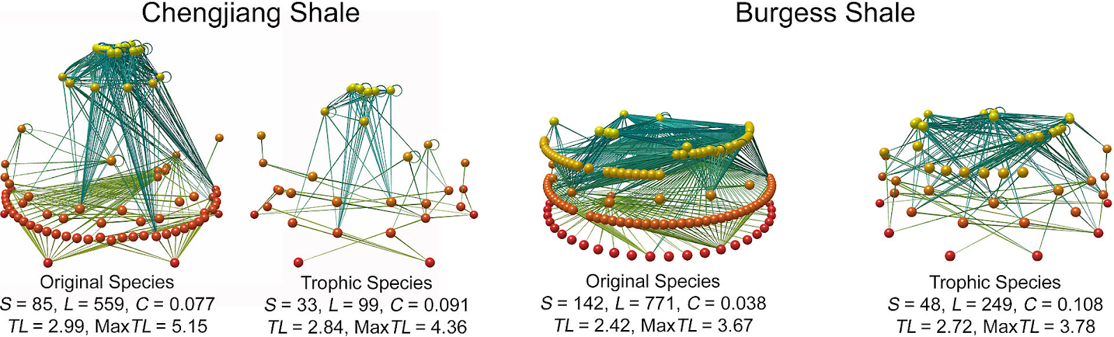
Figure \(\PageIndex{2}\): Food web and trophic level of the Chengjiang and Burgess Shale. S: number of species (nodes). L: number of trophic links. C: connectance; L/S2. MaxTL: maximum trophic level of a species in the web. Paleoecological studies can reconstruct fossil food-webs and trophic levels. Primary producers form the base (red spheres), predators at top (yellow spheres), the lines represent feeding links. Original food-webs (left) are simplified (right) by aggregating groups feeding on common prey into coarser grained trophic species (Dunne et al., 2008). Figure developed by Dunne et al. 2008 is licensed under CC-BY 4.0.
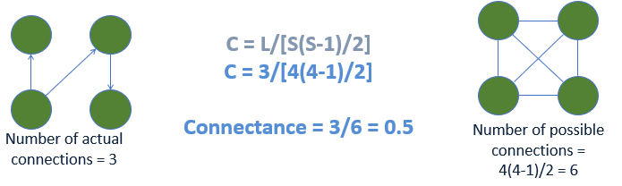
Figure \(\PageIndex{3}\): Worked example of calculating connectance for a food web. Diagram by N. Gownaris and A. Wilson.
Food web linkages, or the feeding relationships between species inhabiting a shared ecosystem, are an ecological lens through which ecosystem structure and function can be assessed, and thus are fundamental to informing sustainable resource management. Empirical feeding datasets have traditionally been painstakingly generated from stomach content analysis, direct observations and from biochemical trophic markers (stable isotopes, fatty acids, molecular tools). Each approach carries inherent biases and limitations, as well as advantages.
Traditional Approaches to Studying Food Webs
Traditional approaches to food web analysis include gut and scat content analysis. In these analyses, the diet of species is determined based on the remains of prey found in their stomachs or in their feces. These approaches are limited because they only allow researchers to examine the hard parts or otherwise undigested components of prey (e.g., otoliths, or ear bones, of fish and teeth of mice). Over the past two decades, stable isotope analysis has become an increasingly common approach to studying food webs. Even more recently, two new methods to studying food webs have emerged: the use of remotely operated vehicles and the use of DNA in feces and gut contents. Below, we provide an example of a recent study using remotely operated vehicles to study food webs and diet in the deep sea.
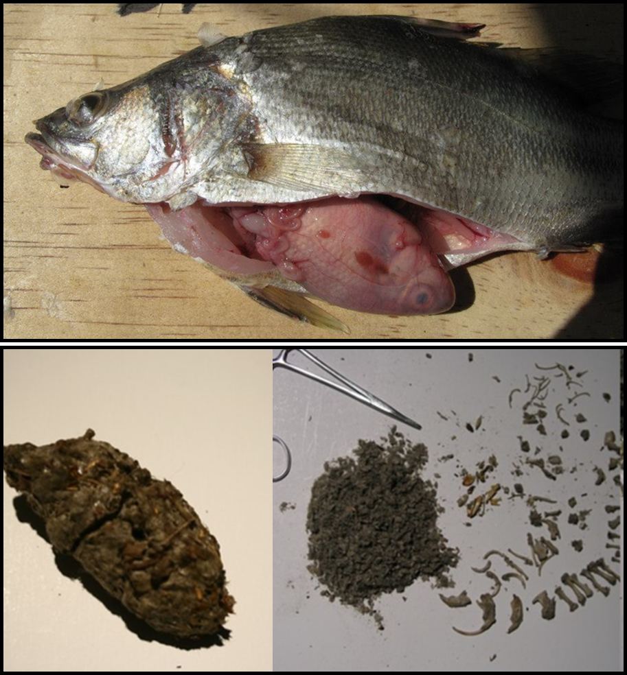
Figure \(\PageIndex{4}\): Traditional food web analysis has often entailed gut content analysis or fecal content analysis. Scientists use the bits of prey that remain to calculate estimates of variables like percent occurrence for each prey type. The top photo (taken by N. Gownaris, licenced CC-BY) shows a tilapia in the stomach of a Nile perch; very rarely is gut content analysis this straightforward! The bottom photo (inside the owl pellet by Art Siegel and licensed under CC-BY-NC 2.0) shows prey remains removed from an owl pellet, including teeth, claws, and bones of owl prey.
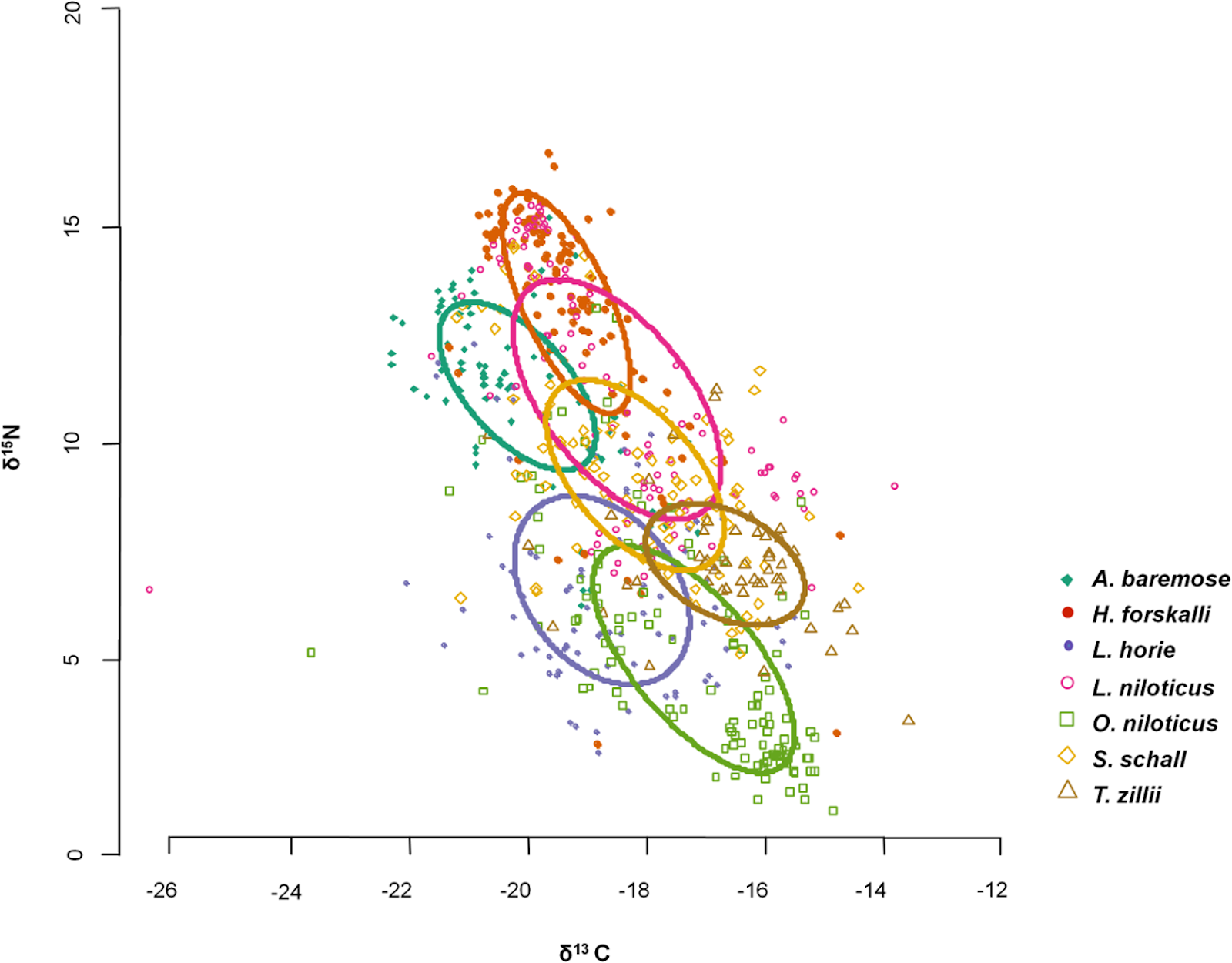
Figure \(\PageIndex{5}\): An example of a food web study using stable isotopes of seven key fish species in Lake Turkana, Kenya. In stable isotope studies, δ13C provides information on the foraging habitat of each species, while δ15N provides information on the trophic level. Species foraging more offshore or more pelagically have a lower δ13C signature and species feeding at lower trophic levels have a lower δ15N signature. In this example, H. forskalii is a pelagic fish (i.e., it feeds in the lake’s open waters) and has the highest trophic level among the species studied. Figure from Gownaris et al., 2015.
The Use of Remotely Operated Vehicles to Understand Understudied Food Webs
Within the deep sea, Earth's largest ecosystem, the challenge of gathering empirical feeding data for food webs is particularly formidable due to logistical access and sampling constraints (Robison, 2004). Analyzing the contents of a consumer's stomach (gut or stomach content analysis) is the common and most directly quantitative way of inferring diet, and is an irreplaceable approach for determining the taxonomic identity of food web components. However, for deeper-dwelling fishes with internal gas spaces, stomach eversion can confound this approach (Drazen & Sutton, 2017). These analyses may also fail to quantify gelatinous prey that are readily digested and become quickly unrecognizable (Hyslop, 1980; Choy, 2013).

Figure \(\PageIndex{6}\): A suite of six illustrative ROV frame grabs of pelagic predators and their prey included in Choy et al. (2017). No scale bars for size are available from these sequences. From left to right, top to bottom: (a) Gonatus sp. (squid) feeding on a bathylagid fish (Bathylagidae); (b) Periphylla periphylla, the helmet jellyfish, feeding on a gonatid squid (Gonatidae), with a small narcomedusa (Aegina sp.) also captured; (c) an undescribed physonect siphonophore known as ‘the galaxy siphonophore’ feeding on a lanternfish of the family Myctophidae; (d) a narcomedusa, Solmissus, ingesting a salp chain (Salpida); (e) the ctenophore Thalassocalyce inconstans, with a euphausiid (Euphausiacea) in its gut; and (f) the trachymedusa, Halitrephes maasi, with a large, red mysid (Mysidae) in its gut. Figure from Choy et al., 2017.
Choy et al. (2017) used 27 years (1991–2016) of in situ feeding observations collected by remotely operated vehicles (ROVs) to quantitatively characterize the deep pelagic food web of central California within the California Current, complementing existing studies of diet and trophic interactions with a unique perspective. Seven hundred and forty-three independent feeding events were observed with ROVs from near-surface waters down to depths approaching 4000 m, involving an assemblage of 84 different predators and 82 different prey types, for a total of 242 unique feeding relationships. The greatest diversity of prey was consumed by narcomedusae, followed by physonect siphonophores, ctenophores and cephalopods. This study highlighted key interactions within the poorly understood ‘jelly web’, showing the importance of medusae, ctenophores and siphonophores as key predators, whose ecological significance is comparable to large fish and squid species within the central California deep pelagic food web.
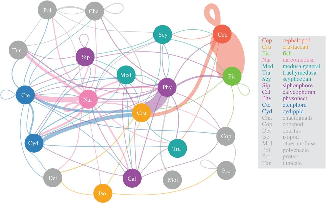
Figure \(\PageIndex{7}\): An in situ perspective of the food web derived from ROV-based observations of feeding, as represented by 20 broad taxonomic groupings. The linkages between predator to prey are coloured according to predator group origin, and loops indicate within-group feeding. The thickness of the lines or edges connecting food web components is scaled to the log of the number of unique ROV feeding observations across the years 1991–2016 between the two groups of animals. The different groups have eight colour-coded types according to main animal types as indicated by the legend and defined here: red, cephalopods; orange, crustaceans; light green, fish; dark green, medusa; purple, siphonophores; blue, ctenophores and grey, all other animals. In this plot, the vertical axis does not correspond to trophic level, because this metric is not readily estimated for all members. Note that for the Sip and Med groups, there are overlapping sub-groups (calycophoran and physonect siphonophores, and trachymedusa and scyphozoan medusa, respectively), which is attributed to varying levels of taxonomic discrimination possible from in situ video observations. Figure from Choy et al., 2017.