9.3: Population Dynamics and Regulation

How do populations change?

Changes in population size over time and the processes that cause these to occur are called population dynamics. How populations change in abundance over time is a major concern of population ecology, wildlife ecology, and conservation biology, and is related to questions asked in evolutionary biology. The processes and mechanisms that drive population change are varied and include intraspecific competition with members of the same population, interspecific competition between species, the availability of food or other resources, extreme weather, inbreeding, predators or parasites.

Populations are dynamic and frequently change size, density, or spatial extent

We can consider changes in populations from multiple angles. For example, Kirtland’s Warbler (Setophaga kirtlandii) in North America is currently:

1. Increasing in the overall number of individuals (population size).

2. Increasing in the number of occupied habitat patches (occupancy).

3. Increasing in the geographic area it occurs in (population distribution and species range).

Importantly, since the warbler prefers a certain density of Jack Pine, its density within an occupied habitat also changes. Jack Pine stands are naturally prone to burning in forest fires, and are also logged for timber. As the density of trees changes due to these disturbances, the density of warblers changes. After a fire or logging there are few if any mature pine trees and therefore few warblers.  Approximately five years after seedlings have sprouted and grown up to be the proper size, the density of warblers can increase. When pine forests get too old habitat conditions are not ideal for the warbler and their abundance declines.

Many studies of population growth focus on changes in population size

Though there are many dimensions to spatial and temporal population dynamics, discussions of population dynamics often center on changes in population size over time. Changes in population size are often displayed in a time series graph with time on the x-axis (usually in years) and population size (N) on the y-axis.  General patterns of population dynamics in terms of population size include:

1. Growth: Growing larger than the current size (Snail kites: Figure \(\PageIndex{1}\) Panel A)

2. Decline: Decreasing in abundance (Elk: Figure \(\PageIndex{1}\) Panel B)

3. Stability: Staying approximately the same size over time (Wolves: Figure \(\PageIndex{1}\) Panel C)

4. Recovery: Stability or growth following a period of decline. (Impala: Figure \(\PageIndex{1}\) Panel D). 

5. Extirpation (local extinction): Decline of one or more populations of a species to 0 (Kirtland's Warbler, Figure \(\PageIndex{1}\) Panel A). 

6. Extinction: Decline of all members of a species to 0 (Northern White Rhino, Figure \(\PageIndex{1}\) Panel B).

7. Cycles: repeated patterns of growth followed by decline (Lynx: Figure \(\PageIndex{1}\) Panel C)

 

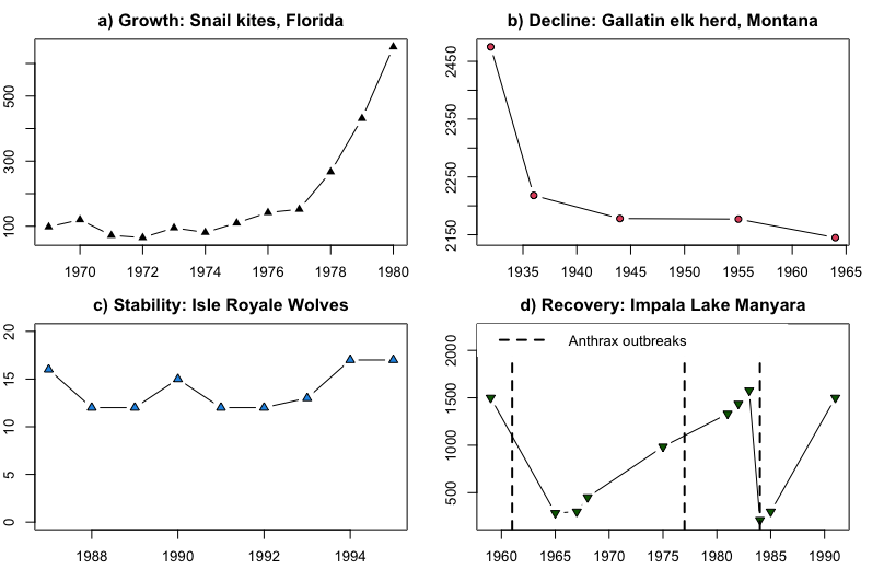
Figure \(\PageIndex{1}\):  Common patterns of population change. The x-axis in all panels is the year and the y-axis is the number of individuals.   a) Growth in a Florida Snail Kite (Rostrhamus sociabilis) population from 1970s to 1980s (Sykes 1983); b) Decline of the Gallatin, Montana herd of elk (Cervus canadensis) from the 1920s to 1960s (Peek et al. 1967); c) Stability of the Isle Royale, Michigan pack of wolves (Canis lupus) in the 1980s and 1990s (Peterson et al. 1998); d) Recovery after population crashes in the Lake Manyara National Park, Tanzania herd of impala (Prins and Weyerhaeuser 1987). 

 

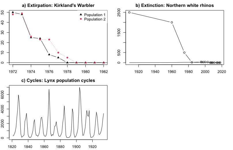
Figure \(\PageIndex{2}\):  Common patterns of population change.   The x-axis in all panels is the year. a) Decline to extirpation (local extinction) of Kirtland's Warbler in two populations (Probst 1986).  The y-axis is the number of singing males; b) Decline to global extinction of the Northern White Rhinoceros (Ceratotherium simum cottoni), one of two subspecies of White Rhinos (Smith 2001, Emslie 2012). The y-axis is the total number of rhinos in the wild. c) Repeated cycling of the Canada lynx (Lynx canadensis; Campbell and Walker 1977). The y-axis is the number of lynx trapped, an index of population size.  

Over the course of many years, a single population can display many of these dynamics.  For example, Kirtland's Warbler populations were monitored by determining the number of males defending territories in their summer breeding habitat in the Great Lakes region North America, primarily Michigan. There were about 500 males with territories in the 1950s (Figure \(\PageIndex{3}\)). The following changes occurred over the next 50 years after the species began being protected by the Endangered Species Act (Kepler et al. 1996):

1. Decline over the course of the 1960s to ~200 territories.

2. A period of stability at ~200 territories from 1975 to 1990.

3. Steady growth to >2500 from 1990 through 2020.

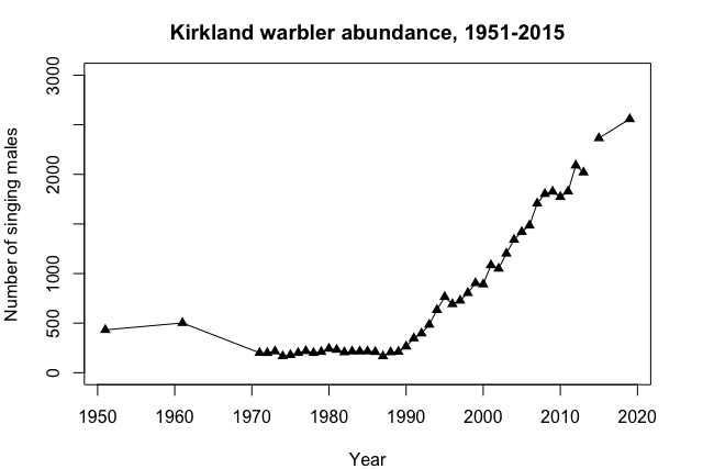
Figure \(\PageIndex{3}\):  Number of singing Kirtland's Warbler (Setophaga kirtlandii) males, 1950 to 2020.

Models can be used to understand and predict population dynamics

Researchers who study population dynamics often use mathematical models to describe and predict population dynamics and understand what factors are driving those changes. For example, if there are 2500 Kirtland’s Warblers in Michigan this year, can we predict how many will be around next year, or 10 years from now? Due to its small population size the Kirtland’s Warbler was listed as an Endangered Species in 1967. In 2019 it was de-listed and now is considered “Near-threatened.” Ecologists are very interested in using models to predict how large the Kirtland’s Warbler population will be in the future, and what factors cause it to increase and decrease (Brown et al. 2019).  In the next chapter we will explore the conceptual and mathematical tools ecologists use to understand population dynamics and predict their future trajectories.

 

Biotic interactions and abiotic conditions limit the sizes of populations

Population dynamics can be regulated in a variety of ways. These are grouped into density-dependent factors, in which the density of the population at a given time affects growth rate and mortality, and density-independent factors, which influence mortality in a population regardless of population density. Note that in the former, the effect of the factor on the population depends on the density of the population at onset. Conservation biologists want to understand both types because this helps them manage populations and prevent extinction or overpopulation.

Density-Dependent Regulation

Most density-dependent factors are biological in nature (biotic), and include predation, inter- and intraspecific competition, accumulation of waste, and diseases such as those caused by parasites. Usually, the denser a population is, the greater its mortality rate. For example, during intra- and interspecific competition, the reproductive rates of the individuals will usually be lower, reducing their population’s rate of growth. In addition, low prey density increases the mortality of its predator because it has more difficulty locating its food source.

An example of density-dependent regulation is shown in Figure \(\PageIndex{4}\) with results from a study focusing on the giant intestinal roundworm (Ascaris lumbricoides), a parasite of humans and other mammals (Croll et al. 1982). Denser populations of the parasite exhibited lower fecundity: they contained fewer eggs. One possible explanation for this is that females would be smaller in more dense populations (due to limited resources) and that smaller females would have fewer eggs. This hypothesis was tested and disproved in a 2009 study which showed that female weight had no influence (Walker et al. 2009). The actual cause of the density-dependence of fecundity in this organism is still unclear and awaiting further investigation.

Figure \(\PageIndex{4}\):  In this population of roundworms Ascaris lumbricoides, fecundity (number of eggs) decreases with population density (Croll et al. 1982).

 

Density-Independent Regulation and Interaction with Density-Dependent Factors

Many factors, typically physical or chemical in nature (abiotic), influence the mortality of a population regardless of its density, including weather, natural disasters, and pollution. An individual deer may be killed in a forest fire regardless of how many deer happen to be in that area. Its chances of survival are the same whether the population density is high or low. The same holds true for cold winter weather.

In real-life situations, population regulation is very complicated and density-dependent and independent factors can interact. A dense population that is reduced in a density-independent manner by some environmental factor(s) will be able to recover differently than a sparse population. For example, a population of deer affected by a harsh winter will recover faster if there are more deer remaining to reproduce.

 

 

Contributors and Attributions

This chapter was written by N. Brouwer with text taken from the following CC-BY resources: 

• OpenStax Biology 2e section 45.4 Population Dynamics and Regulation