
2.7: What Makes the Climate Change
- Page ID
- 78826
\( \newcommand{\vecs}[1]{\overset { \scriptstyle \rightharpoonup} {\mathbf{#1}} } \)
\( \newcommand{\vecd}[1]{\overset{-\!-\!\rightharpoonup}{\vphantom{a}\smash {#1}}} \)
\( \newcommand{\dsum}{\displaystyle\sum\limits} \)
\( \newcommand{\dint}{\displaystyle\int\limits} \)
\( \newcommand{\dlim}{\displaystyle\lim\limits} \)
\( \newcommand{\id}{\mathrm{id}}\) \( \newcommand{\Span}{\mathrm{span}}\)
( \newcommand{\kernel}{\mathrm{null}\,}\) \( \newcommand{\range}{\mathrm{range}\,}\)
\( \newcommand{\RealPart}{\mathrm{Re}}\) \( \newcommand{\ImaginaryPart}{\mathrm{Im}}\)
\( \newcommand{\Argument}{\mathrm{Arg}}\) \( \newcommand{\norm}[1]{\| #1 \|}\)
\( \newcommand{\inner}[2]{\langle #1, #2 \rangle}\)
\( \newcommand{\Span}{\mathrm{span}}\)
\( \newcommand{\id}{\mathrm{id}}\)
\( \newcommand{\Span}{\mathrm{span}}\)
\( \newcommand{\kernel}{\mathrm{null}\,}\)
\( \newcommand{\range}{\mathrm{range}\,}\)
\( \newcommand{\RealPart}{\mathrm{Re}}\)
\( \newcommand{\ImaginaryPart}{\mathrm{Im}}\)
\( \newcommand{\Argument}{\mathrm{Arg}}\)
\( \newcommand{\norm}[1]{\| #1 \|}\)
\( \newcommand{\inner}[2]{\langle #1, #2 \rangle}\)
\( \newcommand{\Span}{\mathrm{span}}\) \( \newcommand{\AA}{\unicode[.8,0]{x212B}}\)
\( \newcommand{\vectorA}[1]{\vec{#1}} % arrow\)
\( \newcommand{\vectorAt}[1]{\vec{\text{#1}}} % arrow\)
\( \newcommand{\vectorB}[1]{\overset { \scriptstyle \rightharpoonup} {\mathbf{#1}} } \)
\( \newcommand{\vectorC}[1]{\textbf{#1}} \)
\( \newcommand{\vectorD}[1]{\overrightarrow{#1}} \)
\( \newcommand{\vectorDt}[1]{\overrightarrow{\text{#1}}} \)
\( \newcommand{\vectE}[1]{\overset{-\!-\!\rightharpoonup}{\vphantom{a}\smash{\mathbf {#1}}}} \)
\( \newcommand{\vecs}[1]{\overset { \scriptstyle \rightharpoonup} {\mathbf{#1}} } \)
\(\newcommand{\longvect}{\overrightarrow}\)
\( \newcommand{\vecd}[1]{\overset{-\!-\!\rightharpoonup}{\vphantom{a}\smash {#1}}} \)
\(\newcommand{\avec}{\mathbf a}\) \(\newcommand{\bvec}{\mathbf b}\) \(\newcommand{\cvec}{\mathbf c}\) \(\newcommand{\dvec}{\mathbf d}\) \(\newcommand{\dtil}{\widetilde{\mathbf d}}\) \(\newcommand{\evec}{\mathbf e}\) \(\newcommand{\fvec}{\mathbf f}\) \(\newcommand{\nvec}{\mathbf n}\) \(\newcommand{\pvec}{\mathbf p}\) \(\newcommand{\qvec}{\mathbf q}\) \(\newcommand{\svec}{\mathbf s}\) \(\newcommand{\tvec}{\mathbf t}\) \(\newcommand{\uvec}{\mathbf u}\) \(\newcommand{\vvec}{\mathbf v}\) \(\newcommand{\wvec}{\mathbf w}\) \(\newcommand{\xvec}{\mathbf x}\) \(\newcommand{\yvec}{\mathbf y}\) \(\newcommand{\zvec}{\mathbf z}\) \(\newcommand{\rvec}{\mathbf r}\) \(\newcommand{\mvec}{\mathbf m}\) \(\newcommand{\zerovec}{\mathbf 0}\) \(\newcommand{\onevec}{\mathbf 1}\) \(\newcommand{\real}{\mathbb R}\) \(\newcommand{\twovec}[2]{\left[\begin{array}{r}#1 \\ #2 \end{array}\right]}\) \(\newcommand{\ctwovec}[2]{\left[\begin{array}{c}#1 \\ #2 \end{array}\right]}\) \(\newcommand{\threevec}[3]{\left[\begin{array}{r}#1 \\ #2 \\ #3 \end{array}\right]}\) \(\newcommand{\cthreevec}[3]{\left[\begin{array}{c}#1 \\ #2 \\ #3 \end{array}\right]}\) \(\newcommand{\fourvec}[4]{\left[\begin{array}{r}#1 \\ #2 \\ #3 \\ #4 \end{array}\right]}\) \(\newcommand{\cfourvec}[4]{\left[\begin{array}{c}#1 \\ #2 \\ #3 \\ #4 \end{array}\right]}\) \(\newcommand{\fivevec}[5]{\left[\begin{array}{r}#1 \\ #2 \\ #3 \\ #4 \\ #5 \\ \end{array}\right]}\) \(\newcommand{\cfivevec}[5]{\left[\begin{array}{c}#1 \\ #2 \\ #3 \\ #4 \\ #5 \\ \end{array}\right]}\) \(\newcommand{\mattwo}[4]{\left[\begin{array}{rr}#1 \amp #2 \\ #3 \amp #4 \\ \end{array}\right]}\) \(\newcommand{\laspan}[1]{\text{Span}\{#1\}}\) \(\newcommand{\bcal}{\cal B}\) \(\newcommand{\ccal}{\cal C}\) \(\newcommand{\scal}{\cal S}\) \(\newcommand{\wcal}{\cal W}\) \(\newcommand{\ecal}{\cal E}\) \(\newcommand{\coords}[2]{\left\{#1\right\}_{#2}}\) \(\newcommand{\gray}[1]{\color{gray}{#1}}\) \(\newcommand{\lgray}[1]{\color{lightgray}{#1}}\) \(\newcommand{\rank}{\operatorname{rank}}\) \(\newcommand{\row}{\text{Row}}\) \(\newcommand{\col}{\text{Col}}\) \(\renewcommand{\row}{\text{Row}}\) \(\newcommand{\nul}{\text{Nul}}\) \(\newcommand{\var}{\text{Var}}\) \(\newcommand{\corr}{\text{corr}}\) \(\newcommand{\len}[1]{\left|#1\right|}\) \(\newcommand{\bbar}{\overline{\bvec}}\) \(\newcommand{\bhat}{\widehat{\bvec}}\) \(\newcommand{\bperp}{\bvec^\perp}\) \(\newcommand{\xhat}{\widehat{\xvec}}\) \(\newcommand{\vhat}{\widehat{\vvec}}\) \(\newcommand{\uhat}{\widehat{\uvec}}\) \(\newcommand{\what}{\widehat{\wvec}}\) \(\newcommand{\Sighat}{\widehat{\Sigma}}\) \(\newcommand{\lt}{<}\) \(\newcommand{\gt}{>}\) \(\newcommand{\amp}{&}\) \(\definecolor{fillinmathshade}{gray}{0.9}\)There are two parts to climate change, the first one is known as climate forcing, which is when conditions change to give the climate a little nudge in one direction or the other. The second part of climate change, and the one that typically does most of the work, is what we call a feedback. When a climate forcing changes the climate a little, a whole series of environmental changes take place, many of which either exaggerate the initial change (positive feedbacks), or suppress the change (negative feedbacks). In this section we will be discussing primarily natural climate forcing. Natural climate forcing has been going on throughout geological time. A wide range of processes has been operating at widely different time scales, from a few years to billions of years.
An example of a climate-forcing mechanism is the increase in the amount of carbon dioxide (CO2) in the atmosphere that results from our use of fossil fuels. CO2 traps heat in the atmosphere and leads to climate warming. Warming changes vegetation patterns; contributes to the melting of snow, ice, and permafrost; causes sea level to rise; reduces the solubility of CO2 in sea water; and has a number of other minor effects. Most of these changes contribute to more warming. Melting of permafrost, for example, is a strong positive feedback because frozen soil contains trapped organic matter that is converted to CO2 and methane (CH4) when the soil thaws. Both these gases accumulate in the atmosphere and add to the warming effect. On the other hand, if warming causes more vegetation growth, that vegetation should absorb CO2, thus reducing the warming effect, which would be a negative feedback. Under our current conditions—a planet that still has lots of glacial ice and permafrost—most of the feedbacks that result from a warming climate are positive feedbacks and so the climate changes that we cause get naturally amplified by natural processes.
Natural Climate Forcing
Life Cycle of the Sun
The longest-term natural forcing variation is related to the evolution of the Sun. Like most other stars of a similar mass, our Sun is evolving. For the past 4.57 billion years, its rate of nuclear fusion has been increasing, and it is now emitting about 40% more energy (as light) than it did at the beginning of geological time (Figure \(\PageIndex{1}\)). A difference of 40% is big, so it’s a little surprising that the temperature on Earth has remained at a reasonable and habitable temperature for all of this time. The mechanism for that relative climate stability has been the evolution of our atmosphere from one that was dominated by CO2, and also had significant levels of CH4—both GHGs—to one with only a few hundred parts per million of CO2 and just under 1 part per million of CH4 because, over geological time, life and its metabolic processes have evolved and changed the atmosphere.

Figure \(\PageIndex{1}\): The life cycle of our Sun and of other similar stars. Source: image
“Solar Life Cycle” by Oliver Beatson is available in the public domain.
Changes occurring in the sun itself can affect the intensity of the sunlight that reaches Earth’s surface. The intensity of the sunlight can cause either warming (during periods of stronger solar intensity) or cooling (during periods of weaker solar intensity). The sun follows a natural 11-year cycle of small ups and downs in intensity, but the effect of these 11-year cycles on Earth’s climate is small.
Milankovitch Cycles
Earth’s orbit around the Sun is nearly circular, but like all physical systems, it has natural oscillations (Figure \(\PageIndex{2}\)). The importance of changes in the eccentricity (shape) of the Earth's orbit, tilt of the Earth, and precession (where the Earth's axis points) to Earth’s climate cycles (now known as Milankovitch Cycles) was first pointed out by Yugoslavian engineer and mathematician Milutin Milankovitch in the early 1900s. Milankovitch recognized that although the variations in the orbital cycles did not affect the total amount of insolation (light energy from the Sun) that Earth received, it did affect where on Earth that energy was strongest. Glaciations are most sensitive to the insolation received at latitudes of around 65°, and with the current configuration of continents, it would have to be 65° north (because there is almost no land at 65° south).
First, the shape of the orbit changes on a regular time scale — close to 100,000 years — from being close to circular to being very slightly elliptical. But the circularity of the orbit is not what matters; it is the fact that as the orbit becomes more elliptical, the position of the Sun within that ellipse becomes less central or more eccentric (Figure \(\PageIndex{2}\)a). Eccentricity is important because when it is high, the Earth-Sun distance varies more from season to season than it does when eccentricity is low.

Figure \(\PageIndex{2}\): The cycles of Earth’s orbit and rotation. These are also called the Milankovitch Cycles. Source: Steven Earle, licensed under CC BY.
Second, Earth rotates around an axis through the North and South Poles, and that axis is at an angle to the plane of Earth’s orbit around the Sun (Figure \(\PageIndex{2}\)b). The angle of tilt (also known as obliquity) varies on a time scale of 41,000 years. When the angle is at its maximum (24.5°), Earth’s seasonal differences are accentuated. When the angle is at its minimum (22.1°), seasonal differences are minimized. The current hypothesis is that glaciation is favored at low seasonal differences as summers would be cooler and snow would be less likely to melt and more likely to accumulate from year to year.
Third, the direction in which Earth’s rotational axis points also varies, on a time scale of about 20,000 years (Figure \(\PageIndex{2}\)c). This variation, known as precession, means that although the North Pole is presently pointing to the star Polaris (the pole star), in 10,000 years it will point to the star Vega.
The most important aspects are whether the northern hemisphere is pointing toward the Sun at its closest or farthest approach, and how eccentric the Sun’s position is in Earth’s orbit. Two opposing situations are when the northern hemisphere is at its farthest distance from the Sun during summer, which means cooler summers, and when the northern hemisphere is at its closest distance to the Sun during summer, which means hotter summers. Cool summers—as opposed to cold winters—are the key factor in the accumulation of glacial ice, so the scenario where the northern hemisphere is at its farthest distance from the Sun during summer is the one that promotes glaciation. This factor is greatest when eccentricity is high (so the difference between the closest point to the Sun and furthest point from the Sun is larger). For a more detailed explanation on Mikankovich Cycles see Milankovitch.
As already stated, climate feedbacks are critically important in amplifying weak climate forcings into full-blown climate changes. When Milankovitch published his hypothesis in 1924, it was widely ignored, partly because it was evident to climate scientists that the forcing produced by the orbital variations was not strong enough to drive the significant climate changes of the glacial cycles. Those scientists did not recognize the power of positive feedbacks. It was not until 1973, 15 years after Milankovitch’s death, that sufficiently high-resolution data were available to show that the Pleistocene glaciations were indeed driven by the orbital cycles, and it became evident that the orbital cycles were just the forcing that initiated a range of feedback mechanisms that made the climate change.
Data for tilt, eccentricity, and precession over the past 400,000 years have been used to determine the insolation levels at 65° north, as shown in Figure \(\PageIndex{4}\). Also shown in Figure \(\PageIndex{4}\) are Antarctic ice-core temperatures from the same time period. The correlation between the two is clear, and it shows up in the Antarctic record because when insolation changes lead to growth of glaciers in the northern hemisphere, southern-hemisphere temperatures are also affected.
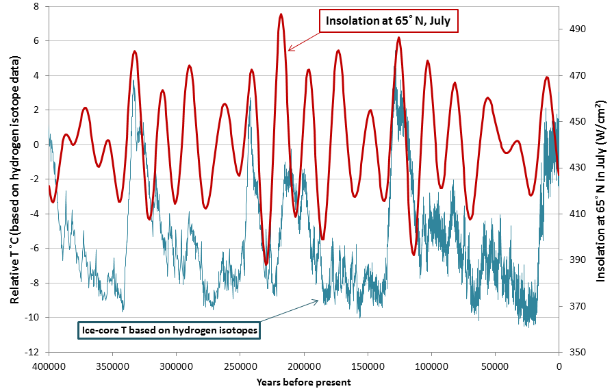
Figure \(\PageIndex{4}\): Insolation at 65° N in July compared with Antarctic ice-core temperatures.
Source: Steven Earle, licensed under CC BY. Based on data from Valerie Masson-Delmotte, “EPICA Dome C Ice Core 800KYr Deuterium Data and Temperature Estimates,” WDCA Contribution Series Number : 2007 -091, NOAA/NCDC Paleoclimatology Program, Boulder CO, USA. Retrieved from: NOAA and from Berger, A. and Loutre, M.F. (1991). Insolation values for the climate of the last 10 million years. Quaternary Science Reviews, 10, 297-317.
Plate Tectonic Processes
Plate tectonic processes contribute to climate forcing in several different ways, and on time scales ranging from tens of millions to hundreds of millions of years. One mechanism is related to continental position. For example, we know that Gondwana (South America + Africa + Antarctica + Australia) was positioned over the South Pole between about 450 and 250 Ma, during which time there were two major glaciations (Andean-Saharan and Karoo) affecting the South polar regions and cooling the rest of the planet at the same time. Another mechanism is related to continental collisions. For example, the collision between India and Asia, which started at around 50 Ma, resulted in massive tectonic uplift. The consequent accelerated weathering of this rugged terrain consumed CO2 from the atmosphere and contributed to gradual cooling over the remainder of the Cenozoic. Changes in continental position can also lead to changes in ocean circulation, and therefore the distribution of energy from equator to the poles. For example, the opening of the Drake Passage — due to plate-tectonic separation of South America from Antarctica — led to the development of the Antarctic Circumpolar Current, which isolated Antarctica from the warmer water in the rest of the ocean and thus contributed to Antarctic glaciation starting at around 35 Ma.

Figure \(\PageIndex{5}\): A map showing 15 of the Earth’s tectonic plates and the approximate rates and directions of plate motions. Source: image "Tectonic Plates" by USGS is available in the public domain and was adapted by Steven Earle.
Volcanic eruptions don’t just involve lava flows and exploding rock fragments; various particulates and gases are also released, including carbon dioxide, water vapor, sulfur dioxide, hydrogen sulfide, hydrogen, and carbon monoxide. Volcanic eruptions can last a few days, but the solids and gases released during an eruption can influence the climate over a period of a few years, causing short-term climate changes. Generally, volcanic eruptions cool the climate. Sulphur dioxide is an aerosol that reflects incoming solar radiation and has a net cooling effect that is short-lived (a few years in most cases, as the particulates settle out of the atmosphere within a couple of years), and doesn’t typically contribute to longer-term climate change. This occurred in 1783 when volcanoes in Iceland erupted and caused the release of large volumes of sulfuric oxide. This led to haze-effect cooling, a global phenomenon that occurs when dust, ash, or other suspended particles block out sunlight and trigger lower global temperatures as a result; haze-effect cooling usually extends for one or more years. In Europe and North America, haze-effect cooling produced some of the lowest average winter temperatures on record in 1783 and 1784. Volcanic CO2 emissions can contribute to climate warming but only if a greater-than-average level of volcanism is sustained over a long time (at least tens of thousands of years). It is widely believed that the catastrophic end-Permian extinction (at 250 Ma) resulted from warming initiated by the eruption of the massive Siberian Traps over a period of at least a million years.
Greenhouse Gas Concentrations
Since scientists cannot go back in time to directly measure climatic variables, such as average temperature and precipitation, they must instead indirectly measure temperature. Antarctic ice cores are a key example of such evidence. These ice cores are samples of polar ice obtained by means of drills that reach thousands of meters into ice sheets or high mountain glaciers. Viewing the ice cores is like traveling backwards through time; the deeper the sample, the earlier the time period. Trapped within the ice are bubbles of air and other biological evidence that can reveal temperature and carbon dioxide data. Antarctic ice cores have been collected and analyzed to indirectly estimate the temperature of the Earth over the past 400,000 years (Figure \(\PageIndex{6}\)a). The 0 °C on this graph refers to the long-term average. Temperatures that are greater than 0 °C exceed Earth’s long-term average temperature. Conversely, temperatures that are less than 0 °C are less than Earth’s average temperature. This figure shows that there have been periodic cycles of increasing and decreasing temperature.
Before the late 1800s, the Earth has been as much as 9 °C cooler and about 3 °C warmer. Note that the graph in Figure \(\PageIndex{6}\)b shows that the atmospheric concentration of carbon dioxide has also risen and fallen in periodic cycles; note the relationship between carbon dioxide concentration and temperature. Figure \(\PageIndex{6}\)b shows that carbon dioxide levels in the atmosphere have historically cycled between 180 and 300 parts per million (ppm) by volume.
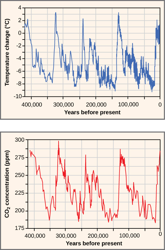
Figure \(\PageIndex{6}\): Ice at the Russian Vostok station in East Antarctica was laid down over the course 420,000 years and reached a depth of over 3,000 m. By measuring the amount of CO2 trapped in the ice, scientists have determined past atmospheric CO2 concentrations. Temperatures relative to modern day were determined from the amount of deuterium (an isotope of hydrogen) present.
Changes in Ocean Currents
Ocean currents are important to climate, and currents also have a tendency to oscillate. Glacial ice cores show clear evidence of changes in the Gulf Stream (and other parts of the thermohaline circulation system) that affected global climate on a time scale of about 1,500 years during the last glaciation.
The east-west changes in sea-surface temperature and surface pressure in the equatorial Pacific Ocean—known as the El Niño Southern Oscillation or ENSO—varies on a much shorter time scale of between two and seven years. These variations tend to garner the attention of the public because they have significant climate implications in many parts of the world. The past 65 years of ENSO index values are shown in Figure \(\PageIndex{7}\). The strongest El Niños in recent decades were in 1983 and 1998, and those were both very warm years from a global perspective. During a strong El Niño, the equatorial Pacific sea-surface temperatures are warmer than normal and heat the atmosphere above the ocean, which leads to warmer-than-average global temperatures.

Figure \(\PageIndex{7}\): Variations in the ENSO index from 1950 to early-2019. Source: Steven Earle with NOAA ("Multivariate ENSO Index (MEI)."
For more information on El Niño and La Niña, see the section of Dr. Paul Webb's Oceanography book on El Niño and La Niña.
Contributors and Attributions
This page was modified from the following sources by Kyle Whittinghill (University of Pittsburgh).
Connie Rye (East Mississippi Community College), Robert Wise (University of Wisconsin, Oshkosh), Vladimir Jurukovski (Suffolk County Community College), Jean DeSaix (University of North Carolina at Chapel Hill), Jung Choi (Georgia Institute of Technology), Yael Avissar (Rhode Island College) among other contributing authors. Original content by OpenStax (CC BY 4.0; Download for free at http://cnx.org/contents/185cbf87-c72...f21b5eabd@9.87).
- Contributed by Melissa Ha and Rachel Schleiger Faculty (Biological Sciences) at Yuba College & Butte College
- Contributed by Paul Webb Professor (Biology) at Rodger Williams University
- Contributed by Chris Johnson, Matthew D. Affolter, Paul Inkenbrandt, & Cam Mosher Faculty (Geology) at Salt Lake Community College
- Contributed by Steven Earle Faculty (Geology) at Vancover Island University
- 19.1 What Makes Climate Change from Physical Geology by Steven Earle (licensed under CC-BY)
- Sourced from OpenGeology from An Introduction to Geology Section 15.2 Earth's Temperature
- 8.1 Earth's Heat Budget from Introduction to Oceanography by Paul Webb (licensed under CC-BY)
- Climate and the Effects of Global Climate Change from General Biology by OpenStax (licensed under CC-BY)
- Climate Change from Environmental Biology by Matthew R. Fisher (licensed under CC-BY)
- Fundamentals of Plate Tectonics from Physical Geology by Steven Earle (licensed under a Creative Commons Attribution 4.0 International License)