21.2: Exercise

Part 1: Natural Selection Exercise—Generation 1

This exercise illustrates the effect of natural selection on populations of predators and prey. Students will represent predators, each with a different adaptation for capturing their prey. The prey will consist of different species represented by different colored beans.

Procedure:

1. Each team of 4 students will count out exactly 100 dried beans of each color.
2. Thoroughly mix the beans and spread them evenly over your “habitat.” Your habitat depends on the weather.
   1. If the weather is poor, it is dark outside, or your instructor would rather, your habitat will be a tray of sediment in the classroom.
   2. If the weather is lovely, or your instructor is adventurous, you will do this lab outside. Each team will mark off a 1m × 1m “habitat” in the grass using yarn, a meter stick, and wood stakes.
   3. All “preys” are confined to the habitat, wherever it is!
3. Each student (predator) will have a different feeding apparatus: A fork, spoon, knife or forceps.

Before you begin, hypothesize which predator will be the most successful. Hypothesize which prey species will be the most successful. As with all hypotheses, be sure to include a reason for your thoughts. Write these two hypotheses down in your lab notebook.

1. When everyone is ready, predators will spend 60 seconds capturing prey with their devices and depositing them into a cup while obeying the following rules:
   1. Predators must only use their capture device to capture prey.
   2. Predators may not scoop prey up with their cup.
   3. If predators “eat” too much of the environment, they will become constipated and DIE.
2. Each predator determines the number of prey captured and records results in Data Sheet: Generation 1.
3. Calculate and fill in the remaining statistics on the data sheet (see example below).

Data Sheet: Generation 1

Data Sheet: Generation 1

Prey Type	Black bean	Pinto bean	Red bean	White bean	Total	% Captured
Population Size	100	100	100	100	400	—
Forceps
Spoon
Fork
Knife

Prey Type	Black bean	Pinto bean	Red bean	White bean	Total	% Captured
Total Kills
# Survived
% Survived
% Total Population

Example of Data Collection and Analysis for Generation 1

Prey Type	Black bean	Pinto bean	Red bean	White bean	Total	% Captured
Population Size	100	100	100	100	400	—
Forceps	8	15	22	12	57	14%
Spoon	14	29	21	18	82	21%
Fork	10	20	14	19	63	15%
Knife	15	30	20	10	75	19%

Prey Type	Black bean	Pinto bean	Red bean	White bean	Total	% Captured
Total Kills	47^[1]	94	77	59	—	—
# of This Bean That Survived	53^[2]	6	23	41	123^[3]	—
% of This Bean That Survived	53%^[4]	6%	23%	41%	—	—
% Total Population	43%^[5]	5%	19%	3%	—	—

# of This Bean That Survived = population size – total kills

% of This Bean That Survived = (# survived/population size) x 100

% Total Population = (# survived/total survived) x 100

Part 2: Natural Selection Exercise—Generation 2

The predator with the lowest capture percentage will go “extinct” and will not participate in the next exercise. The predator with the highest capture percentage will reproduce itself and the “offspring” will participate in the next exercise. The surviving prey will also survive and reproduce.

Procedure:

1. The person with the lowest capture percentage (as calculated in the previous exercise) will “die” and turn in their feeding device.
2. The person with the highest capture percentage will reproduce by having the “dead” person use their same feeding device in the next round.
   1. If the Fork won the first round and the Spoon lost, then in the second round, there will be two Forks and zero Spoons. There will also be one Knife and one pair of Forceps.
3. Now the surviving prey will reproduce and double.
   1. If there are 40 surviving black beans, you will add another 40 black beans to the habitat, so there are a total of 80 black beans in the habitat for round 2.
4. Repeat the procedure you carried out in Part 1. Collect data for Generation 2.

Data Sheet: Generation 2

Prey Type	Black bean	Pinto bean	Red bean	White bean	Total	% Captured
Population Size	100	100	100	100	400	—
Forceps
Spoon
Fork
Knife

Prey Type	Black bean	Pinto bean	Red bean	White bean	Total	% Captured
Total Kills
# Survived
% Survived
% Total Population

Note

For population size in generation 2, multiply the number that survived in generation 1 by two.

Part 3: Natural Selection Exercise—Generation 3

The winning predator will reproduce again and the surviving prey will also reproduce (just like they did in the previous exercise). Collect and record new data.

Data Sheet: Generation 3

Prey Type	Black bean	Pinto bean	Red bean	White bean	Total	% Captured
Population Size	100	100	100	100	400	—
Forceps
Spoon
Fork
Knife

Prey Type	Black bean	Pinto bean	Red bean	White bean	Total	% Captured
Total Kills
# Survived
% Survived
% Total Population

Note

For population size in generation 2, multiply the number that survived in generation 1 by two.

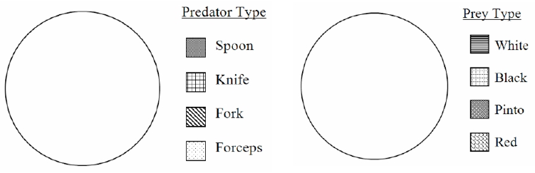
Part 4: Pie Chart Analysis of Predator and Prey Populations

Now that you have collected data from three generations of predator and prey populations, you will use the data to create a set of pie charts to help you interpret your results. The first pair of pie charts represent the data from the original predator and prey populations. Use these examples to create your own charts using your group’s data.

Figure \(\PageIndex{1}\): data from the original predator and prey populations.

End of First Generation:

End of Second Generation:

End of Third Generation:

Questions:

1. Explain in your own words the process of natural selection.
2. What conclusions can you draw regarding the effect of natural selection on the predator populations in this exercise?
3. What conclusions can you draw regarding the effect of natural selection on the prey populations in this exercise?
4. Why did we start with 4 predators but 200 prey? What happen if numbers of predators and prey are equal? Explain
5. Imagine a scenario where the one of the predator groups has very low genetic variability. A disease comes through and modifies the prey-capturing tool, decreasing the predator’s ability to hunt. Predict what would happen to that particular predator group.
6. Relate the concept of natural selection to the process of evolution.
7. Apart from natural selection, the real evolution process will also be influenced by (a) mutations, (b) migrations from other populations and (c) random processes (“genetic drift”). How you would change the rules of game in order to accommodate one or more of these processes?
   • mutations
   • migration
   • genetic drift

---

1. 8 + 14 + 10 +15 ↵
2. 100 – 47 ↵
3. 53 + 6 + 23 + 41 ↵
4. (53/100) × 100 (6/100) × 100 ↵
5. (53/123) × 100 ↵

Licenses and Attributions

CC licensed content, Original

• Biology Labs. Authored by: Wendy Riggs. Provided by: College of the Redwoods. Located at: http://www.redwoods.edu(opens in new window) [www.redwoods.edu] [www.redwoods.edu(opens in new window)]. License: CC BY: Attribution(opens in new window)

Cladistics and Phylogenetics

A new system of phylogenetic classification, called cladistics, is currently in practice today. A cladogram is a hypothesis about the evolutionary relationships between the organisms depicted on the tree. In this way, a cladogram illustrates the lines of descent for these organisms. A cladogram proposes an answer to the question “Which groups of organisms share a common ancestry?”

Take a look at these two identical, generic cladograms. The capital letters indicate the terminal organisms represented in the tree. The numbers indicate characters present in organisms beyond that point. And the nodes (indicated by the lowercase letters and the dots) represent the common ancestors of the terminal organisms. Even though they look different, if you examine them closely, these two cladograms are depicting the same relationships between critters A, B and C.

In this example (Fig 2) you see that A is more closely related to B than C based on the shared derived characteristic 1. Note that at each branch a derived characteristic is indicated that separates the left branch from the right branch of the evolutionary tree.(opens in new window)

Figure \(\PageIndex{2}\): Two cladograms.

Now examine the cladogram at the bottom of this page illustrating the evolutionary relationships between a hagfish, shark, bony fish, frog, rat, bird, and lizard.

Procedure:

1. Name each organism on the cladogram.
2. Place a dot at every point that represents a common ancestor.
3. Indicate one shared derived characteristic that distinguishes each branch.
4. Who is more closely related: the shark and bony fish, or the bony fish and frog?

Figure \(\PageIndex{3}\): Cladogram for Subphylum Vertebrata.

Phylogenetics of Metal Objects

Define phylogenetics

You'll be provided with a set of metal objects. With your group, create a tree/cladogram of the proposed evolutionary relationships between your objects.

You may receive some or all of the following objects:
• 75 mm tack [A]
• 20 mm nail [B]
• 20 mm screw [C]
• Hairpin (50 mm) [D]
• Staple (25 mm) [E]
• Safety pin (40 mm) [F]
• Split rivet (20 mm) [G]
• Paperclip (32 mm) [H]
• 25 mm tack [J]
• Upholstery pin (20 mm) [K]
• 13 mm nail [L]
• Mirror screw (20 mm) [M]
• Insulated staple (13 mm) [N]
• Round-headed paper fastener (20 mm) [O]
• Flat-headed paper fastener (20 mm) [P]
• Round-headed screw (25 mm) [Q]
• 50 mm nail [R]
• Drawing pin (6 mm) [S]
• Hook (20 mm) [T]
• Kirby grip [W]
• Bolt (65 mm) [Z]

Questions:

1. What object did you choose for your common ancestor? Why?
2. Record your tree.
3. Choose one path and explain the sequence of events/line that led to the “most recent” object. For example, L → B → R is a line that depicts an increase in size.
4. Does your tree illustrate an example of convergent evolution? Explain.