10.3: Measurement of Bacterial Growth

Learning Objectives

• Explain several laboratory methods used to determine viable and total cell counts in populations undergoing exponential growth
• Differentiate between direct and indirect methods used to measure bacterial growth
• Explain the principle of viable plate count methods including serial dilution and colony-forming units (CFUs)
• Compare the accuracy, sensitivity and applications of direct counts, plate counts and turbidity-based methods

Measurement of Bacterial Growth

Estimating the number of bacterial cells in a sample, known as a bacterial count, is a common task performed by microbiologists. The number of bacteria in a clinical sample serves as an indication of the extent of an infection. Quality control of drinking water, food, medication, and even cosmetics relies on estimates of bacterial counts to detect contamination and prevent the spread of disease. Two major approaches are used to measure cell number. The direct methods involve counting cells, whereas the indirect methods depend on the measurement of cell presence or activity without actually counting individual cells. Both direct and indirect methods have advantages and disadvantages for specific applications.

Direct Cell Count

Direct cell count refers to counting the cells in a liquid culture or colonies on a plate. It is a direct way of estimating how many organisms are present in a sample. Let’s look first at a simple and fast method that requires only a specialized slide and a compound microscope.

The simplest way to count bacteria is called the direct microscopic cell count, which involves transferring a known volume of a culture to a calibrated slide and counting the cells under a light microscope. The calibrated slide is called a Petroff-Hausser chamber (Figure \(\PageIndex{7}\)) and is similar to a hemocytometer used to count red blood cells. The central area of the counting chamber is etched into squares of various sizes. A sample of the culture suspension is added to the chamber under a coverslip that is placed at a specific height from the surface of the grid. It is possible to estimate the concentration of cells in the original sample by counting individual cells in a number of squares and determining the volume of the sample observed. The area of the squares and the height at which the coverslip is positioned are specified for the chamber. The concentration must be corrected for dilution if the sample was diluted before enumeration.

Figure \(\PageIndex{7}\): (a) A Petroff-Hausser chamber is a special slide designed for counting the bacterial cells in a measured volume of a sample. A grid is etched on the slide to facilitate precision in counting. (b) This diagram illustrates the grid of a Petroff-Hausser chamber, which is made up of squares of known areas. The enlarged view shows the square within which bacteria (red cells) are counted. If the coverslip is 0.2 mm above the grid and the square has an area of 0.04 mm², then the volume is 0.008 mm³, or 0.000008 mL. Since there are 10 cells inside the square, the density of bacteria is 10 cells/0.000008 mL, which equates to 1,250,000 cells/mL. (credit a: modification of work by Jeffrey M. Vinocur)

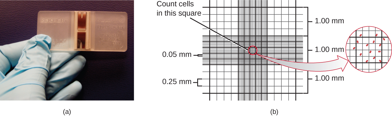
Cells in several small squares must be counted and the average taken to obtain a reliable measurement. The advantages of the chamber are that the method is easy to use, relatively fast, and inexpensive. On the downside, the counting chamber does not work well with dilute cultures because there may not be enough cells to count.

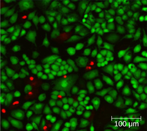
Using a counting chamber does not necessarily yield an accurate count of the number of live cells because it is not always possible to distinguish between live cells, dead cells, and debris of the same size under the microscope. However, newly developed fluorescence staining techniques make it possible to distinguish viable and dead bacteria. These viability stains (or live stains) bind to nucleic acids, but the primary and secondary stains differ in their ability to cross the cytoplasmic membrane. The primary stain, which fluoresces green, can penetrate intact cytoplasmic membranes, staining both live and dead cells. The secondary stain, which fluoresces red, can stain a cell only if the cytoplasmic membrane is considerably damaged. Thus, live cells fluoresce green because they only absorb the green stain, whereas dead cells appear red because the red stain displaces the green stain on their nucleic acids (Figure \(\PageIndex{8}\)).

Figure \(\PageIndex{8}\): Fluorescence staining can be used to differentiate between viable and dead bacterial cells in a sample for purposes of counting. Viable cells are stained green, whereas dead cells are stained red. (credit: modification of work by Panseri S, Cunha C, D’Alessandro T, Sandri M, Giavaresi G, Maracci M, Hung CT, Tampieri A)

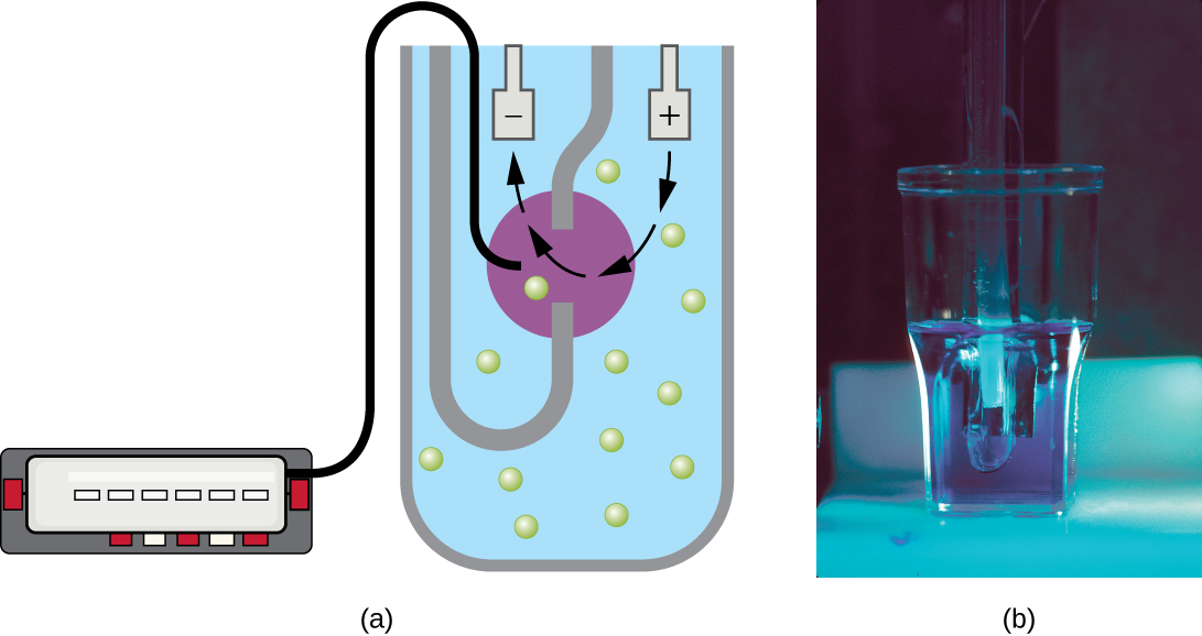
Another technique uses an electronic cell counting device (Coulter counter) to detect and count the changes in electrical resistance in a saline solution. A glass tube with a small opening is immersed in an electrolyte solution. A first electrode is suspended in the glass tube. A second electrode is located outside of the tube. As cells are drawn through the small aperture in the glass tube, they briefly change the resistance measured between the two electrodes and the change is recorded by an electronic sensor (Figure \(\PageIndex{9}\)); each resistance change represents a cell. The method is rapid and accurate within a range of concentrations; however, if the culture is too concentrated, more than one cell may pass through the aperture at any given time and skew the results. This method also does not differentiate between live and dead cells.

Direct counts provide an estimate of the total number of cells in a sample. However, in many situations, it is important to know the number of live, or viable, cells. Counts of live cells are needed when assessing the extent of an infection, the effectiveness of antimicrobial compounds and medication, or contamination of food and water.

Figure \(\PageIndex{9}\): A Coulter counter is an electronic device that counts cells. It measures the change in resistance in an electrolyte solution that takes place when a cell passes through a small opening in the inside container wall. A detector automatically counts the number of cells passing through the opening. (credit b: modification of work by National Institutes of Health)

Query \(\PageIndex{1}\)

 

Plate Count

The viable plate count, or simply plate count, is a count of viable or live cells. It is based on the principle that viable cells replicate and give rise to visible colonies when incubated under suitable conditions for the specimen. The results are usually expressed as colony-forming units per milliliter (CFU/mL) rather than cells per milliliter because more than one cell may have landed on the same spot to give rise to a single colony. Furthermore, samples of bacteria that grow in clusters or chains are difficult to disperse and a single colony may represent several cells. Some cells are described as viable but nonculturable and will not form colonies on solid media. For all these reasons, the viable plate count is considered a low estimate of the actual number of live cells. These limitations do not detract from the usefulness of the method, which provides estimates of live bacterial numbers.

Microbiologists typically count plates with 30–300 colonies. Samples with too few colonies (<30) do not give statistically reliable numbers, and overcrowded plates (>300 colonies) make it difficult to accurately count individual colonies. Also, counts in this range minimize occurrences of more than one bacterial cell forming a single colony. Thus, the calculated CFU is closer to the true number of live bacteria in the population.

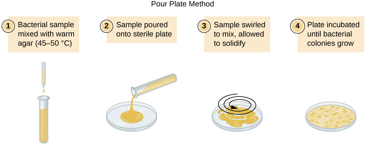
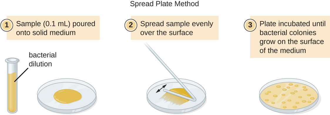
There are two common approaches to inoculating plates for viable counts: the pour plate and the spread plate methods. Although the final inoculation procedure differs between these two methods, they both start with a serial dilution of the culture.

Serial Dilution

The serial dilution of a culture is an important first step before proceeding to either the pour plate or spread plate method. The goal of the serial dilution process is to obtain plates with CFUs in the range of 30–300, and the process usually involves several dilutions in multiples of 10 to simplify calculation. The number of serial dilutions is chosen according to a preliminary estimate of the culture density. Figure \(\PageIndex{10}\) illustrates the serial dilution method.

Figure \(\PageIndex{10}\): Serial dilution involves diluting a fixed volume of cells mixed with dilution solution using the previous dilution as an inoculum. The result is dilution of the original culture by an exponentially growing factor. (credit: modification of work by “Leberechtc”/Wikimedia Commons)

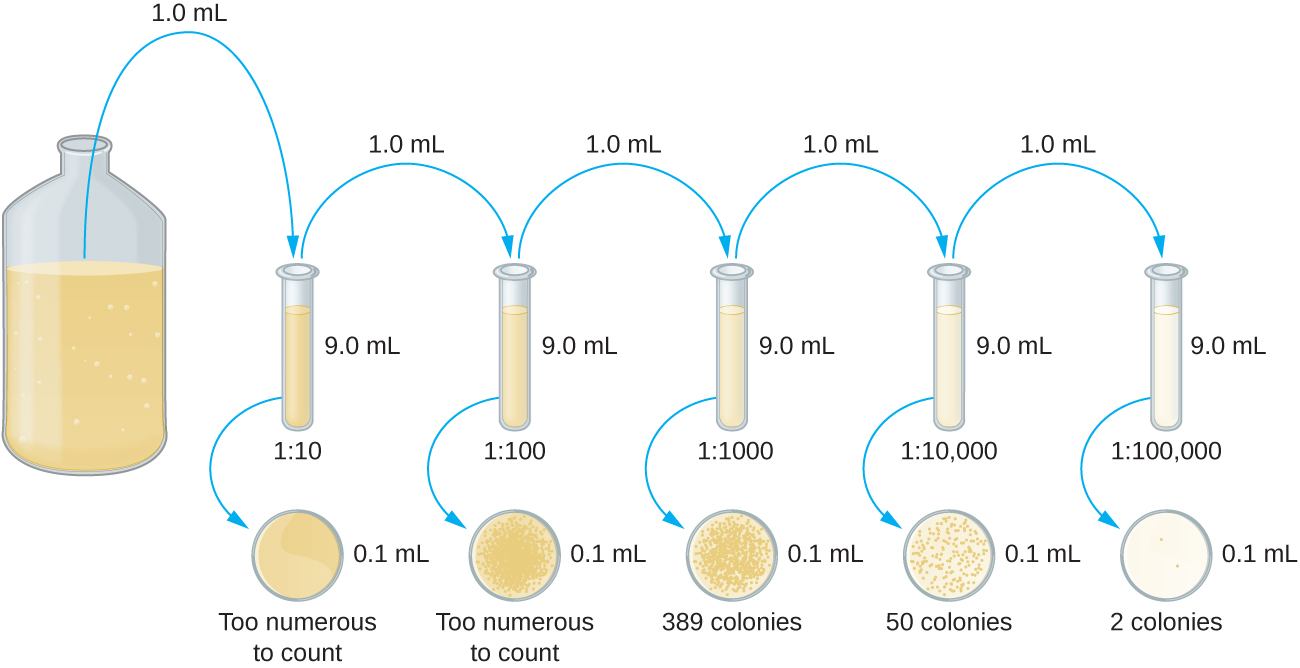
A fixed volume of the original culture, 1.0 mL, is added to and thoroughly mixed with the first dilution tube solution, which contains 9.0 mL of sterile broth. This step represents a dilution factor of 10, or 1:10, compared with the original culture. From this first dilution, the same volume, 1.0 mL, is withdrawn and mixed with a fresh tube of 9.0 mL of dilution solution. The dilution factor is now 1:100 compared with the original culture. This process continues until a series of dilutions is produced that will bracket the desired cell concentration for accurate counting. From each tube, a sample is plated on solid medium using either the pour plate method (Figure \(\PageIndex{11}\)) or the spread plate method (Figure \(\PageIndex{12}\)). The plates are incubated until colonies appear. Two to three plates are usually prepared from each dilution and the numbers of colonies counted on each plate are averaged. In all cases, thorough mixing of samples with the dilution medium (to ensure the cell distribution in the tube is random) is paramount to obtaining reliable results.

Figure \(\PageIndex{11}\): In the pour plate method of cell counting, the sample is mixed in liquid warm agar (45–50 °C) poured into a sterile Petri dish and further mixed by swirling. This process is repeated for each serial dilution prepared. The resulting colonies are counted and provide an estimate of the number of cells in the original volume sampled.

The dilution factor is used to calculate the number of cells in the original cell culture. In our example, an average of 50 colonies was counted on the plates obtained from the 1:10,000 dilution. Because only 0.1 mL of suspension was pipetted on the plate, the multiplier required to reconstitute the original concentration is 10 × 10,000. The number of CFU per mL is equal to 50 × 100 × 10,000 = 5,000,000. The number of bacteria in the culture is estimated as 5 million cells/mL. The colony count obtained from the 1:1000 dilution was 389, well below the expected 500 for a 10-fold difference in dilutions. This highlights the issue of inaccuracy when colony counts are greater than 300 and more than one bacterial cell grows into a single colony.

Figure \(\PageIndex{12}\): In the spread plate method of cell counting, the sample is poured onto solid agar and then spread using a sterile spreader. This process is repeated for each serial dilution prepared. The resulting colonies are counted and provide an estimate of the number of cells in the original volume samples.

A very dilute sample—drinking water, for example—may not contain enough organisms to use either of the plate count methods described. In such cases, the original sample must be concentrated rather than diluted before plating. This can be accomplished using a modification of the plate count technique called the membrane filtration technique. Known volumes are vacuum-filtered aseptically through a membrane with a pore size small enough to trap microorganisms. The membrane is transferred to a Petri plate containing an appropriate growth medium. Colonies are counted after incubation. Calculation of the cell density is made by dividing the cell count by the volume of filtered liquid.

Link to Learning

Watch this video for demonstrations of serial dilutions and spread plate techniques.

In calculating serial dilution, use the equation:

V₁D₁ = V₂D₂

V₁: original volume

D₁: original dilution (undiluted samples are always expressed as 1)

V₂: final volume

D₂: final dilution

Query \(\PageIndex{1}\)

 

The Most Probable Number

The number of microorganisms in dilute samples is usually too low to be detected by the plate count methods described thus far. For these specimens, microbiologists routinely use the most probable number (MPN) method, a statistical procedure for estimating of the number of viable microorganisms in a sample. Often used for water and food samples, the MPN method evaluates detectable growth by observing changes in turbidity or color due to metabolic activity.

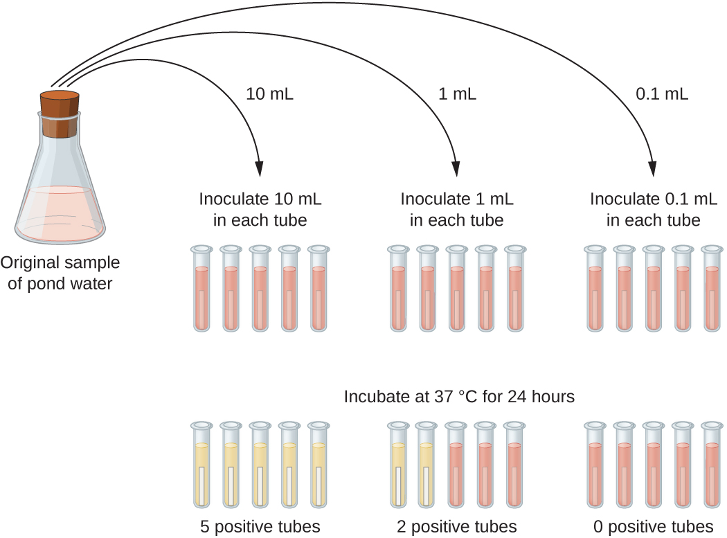
A typical application of MPN method is the estimation of the number of coliforms in a sample of pond water. Coliforms are gram-negative rod bacteria that ferment lactose. The presence of coliforms in water is considered a sign of contamination by fecal matter. For the method illustrated in Figure \(\PageIndex{13}\), a series of three dilutions of the water sample is tested by inoculating five lactose broth tubes with 10 mL of sample, five lactose broth tubes with 1 mL of sample, and five lactose broth tubes with 0.1 mL of sample. The lactose broth tubes contain a pH indicator that changes color from red to yellow when the lactose is fermented. After inoculation and incubation, the tubes are examined for an indication of coliform growth by a color change in media from red to yellow. The first set of tubes (10-mL sample) showed growth in all the tubes; the second set of tubes (1 mL) showed growth in two tubes out of five; in the third set of tubes, no growth is observed in any of the tubes (0.1-mL dilution). The numbers 5, 2, and 0 are compared with Figure B1 in Appendix B, which has been constructed using a probability model of the sampling procedure. From our reading of the table, we conclude that 49 is the most probable number of bacteria per 100 mL of pond water.

Figure \(\PageIndex{13}\): In the most probable number method, sets of five lactose broth tubes are inoculated with three different volumes of pond water: 10 mL, 1 mL, and 0.1mL. Bacterial growth is assessed through a change in the color of the broth from red to yellow as lactose is fermented.

Indirect Cell Counts

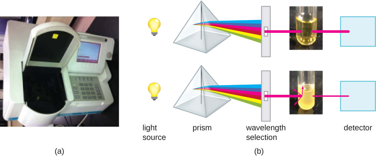
Besides direct methods of counting cells, other methods, based on an indirect detection of cell density, are commonly used to estimate and compare cell densities in a culture. The foremost approach is to measure the turbidity (cloudiness) of a sample of bacteria in a liquid suspension. The laboratory instrument used to measure turbidity is called a spectrophotometer (Figure \(\PageIndex{14}\)). In a spectrophotometer, a light beam is transmitted through a bacterial suspension, the light passing through the suspension is measured by a detector, and the amount of light passing through the sample and reaching the detector is converted to either percent transmission or a logarithmic value called absorbance (optical density). As the numbers of bacteria in a suspension increase, the turbidity also increases and causes less light to reach the detector. The decrease in light passing through the sample and reaching the detector is associated with a decrease in percent transmission and increase in absorbance measured by the spectrophotometer.

Measuring turbidity is a fast method to estimate cell density as long as there are enough cells in a sample to produce turbidity. It is possible to correlate turbidity readings to the actual number of cells by performing a viable plate count of samples taken from cultures having a range of absorbance values. Using these values, a calibration curve is generated by plotting turbidity as a function of cell density. Once the calibration curve has been produced, it can be used to estimate cell counts for all samples obtained or cultured under similar conditions and with densities within the range of values used to construct the curve.

Figure \(\PageIndex{14}\): (a) A spectrophotometer is commonly used to measure the turbidity of a bacterial cell suspension as an indirect measure of cell density. (b) A spectrophotometer works by splitting white light from a source into a spectrum. The spectrophotometer allows choice of the wavelength of light to use for the measurement. The optical density (turbidity) of the sample will depend on the wavelength, so once one wavelength is chosen, it must be used consistently. The filtered light passes through the sample (or a control with only medium) and the light intensity is measured by a detector. The light passing into a suspension of bacteria is scattered by the cells in such a way that some fraction of it never reaches the detector. This scattering happens to a far lesser degree in the control tube with only the medium. (credit a: modification of work by Hwang HS, Kim MS; credit b “test tube photos”: modification of work by Suzanne Wakim)

Measuring dry weight of a culture sample is another indirect method of evaluating culture density without directly measuring cell counts. The cell suspension used for weighing must be concentrated by filtration or centrifugation, washed, and then dried before the measurements are taken. The degree of drying must be standardized to account for residual water content. This method is especially useful for filamentous microorganisms, which are difficult to enumerate by direct or viable plate count.

As we have seen, methods to estimate viable cell numbers can be labor intensive and take time because cells must be grown. Recently, indirect ways of measuring live cells have been developed that are both fast and easy to implement. These methods measure cell activity by following the production of metabolic products or disappearance of reactants. Adenosine triphosphate (ATP) formation, biosynthesis of proteins and nucleic acids, and consumption of oxygen can all be monitored to estimate the number of cells.

Query \(\PageIndex{1}\)

 

Key Concepts and Summary

• Cells can be counted by direct viable cell count. The pour plate and spread plate methods are used to plate serial dilutions into or onto, respectively, agar to allow counting of viable cells that give rise to colony-forming units. Membrane filtration is used to count live cells in dilute solutions. The most probable cell number (MPN)method allows estimation of cell numbers in cultures without using solid media.
• Indirect methods can be used to estimate culture density by measuring turbidity of a culture or live cell density by measuring metabolic activity.