10.2: Growth Curve

Learning Objectives

• Identify and describe the four phases of a typical bacterial growth curve
• Explain the physiological changes that occur in bacterial populations during each phase
• Interpret a bacterial growth curve and correlate it with changes in cell number and metabolic activity

The Growth Curve

Microorganisms grown in closed culture (also known as a batch culture), in which no nutrients are added and most waste is not removed, follow a reproducible growth pattern referred to as the growth curve. An example of a batch culture in nature is a pond in which a small number of cells grow in a closed environment. The culture density is defined as the number of cells per unit volume. In a closed environment, the culture density is also a measure of the number of cells in the population. Infections of the body do not always follow the growth curve, but correlations can exist depending upon the site and type of infection. When the number of live cells is plotted against time, distinct phases can be observed in the curve (Figure \(\PageIndex{4}\)).

Figure \(\PageIndex{4}\): The growth curve of a bacterial culture is represented by the logarithm of the number of live cells plotted as a function of time. The graph can be divided into four phases according to the slope, each of which matches events in the cell. The four phases are lag, log, stationary, and death.

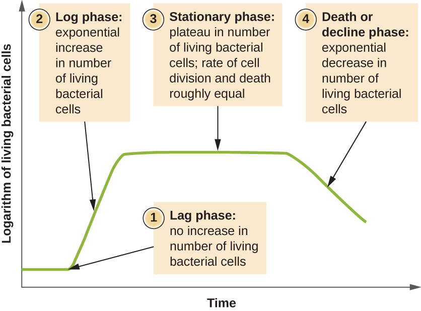
The Lag Phase

The beginning of the growth curve represents a small number of cells, referred to as an inoculum, that are added to a fresh culture medium, a nutritional broth that supports growth. The initial phase of the growth curve is called the lag phase, during which cells are gearing up for the next phase of growth. The number of cells does not change during the lag phase; however, cells grow larger and are metabolically active, synthesizing proteins needed to grow within the medium. If any cells were damaged or shocked during the transfer to the new medium, repair takes place during the lag phase. The duration of the lag phase is determined by many factors, including the species and genetic make-up of the cells, the composition of the medium, and the size of the original inoculum.

The Log Phase

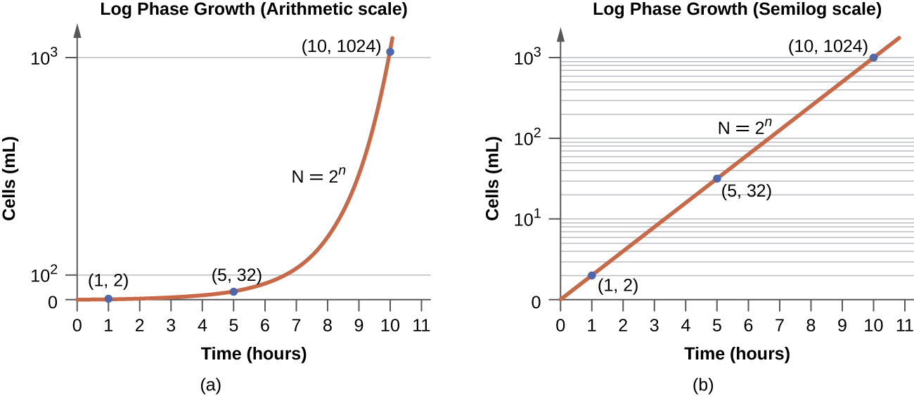
In the logarithmic (log) growth phase, sometimes called exponential growth phase, the cells are actively dividing by binary fission and their number increases exponentially. For any given bacterial species, the generation time under specific growth conditions (nutrients, temperature, pH, and so forth) is genetically determined, and this generation time is called the intrinsic growth rate. During the log phase, the relationship between time and number of cells is not linear but exponential; however, the growth curve is often plotted on a semilogarithmic graph, as shown in Figure \(\PageIndex{5}\), which gives the appearance of a linear relationship.

Figure \(\PageIndex{5}\): Both graphs illustrate population growth during the log phase for a bacterial sample with an initial population of one cell and a doubling time of 1 hour. (a) When plotted on an arithmetic scale, the growth rate resembles a curve. (b) When plotted on a semilogarithmic scale (meaning the values on the y-axis are logarithmic), the growth rate appears linear.

Cells in the log phase show constant growth rate and uniform metabolic activity. For this reason, cells in the log phase are preferentially used for industrial applications and research work. The log phase is also the stage where bacteria are the most susceptible to the action of disinfectants and common antibiotics that affect protein, DNA, and cell-wall synthesis.

Stationary Phase

As the number of cells increases through the log phase, several factors contribute to a slowing of the growth rate. Waste products accumulate and nutrients are gradually used up. In addition, gradual depletion of oxygen begins to limit aerobic cell growth. This combination of unfavorable conditions slows and finally stalls population growth. The total number of live cells reaches a plateau referred to as the stationary phase (Figure \(\PageIndex{4}\)). In this phase, the number of new cells created by cell division is now equivalent to the number of cells dying; thus, the total population of living cells is relatively stagnant. The culture density in a stationary culture is constant. The culture’s carrying capacity, or maximum culture density, depends on the types of microorganisms in the culture and the specific conditions of the culture; however, carrying capacity is constant for a given organism grown under the same conditions.

During the stationary phase, cells switch to a survival mode of metabolism. As growth slows, so too does the synthesis of peptidoglycans, proteins, and nucleic-acids; thus, stationary cultures are less susceptible to antibiotics that disrupt these processes. In bacteria capable of producing endospores, many cells undergo sporulation during the stationary phase. Secondary metabolites, including antibiotics, are synthesized in the stationary phase. In certain pathogenic bacteria, the stationary phase is also associated with the expression of virulence factors, products that contribute to a microbe’s ability to survive, reproduce, and cause disease in a host organism. For example, quorum sensing in Staphylococcus aureus initiates the production of enzymes that can break down human tissue and cellular debris, clearing the way for bacteria to spread to new tissue where nutrients are more plentiful.

The Death Phase

As a culture medium accumulates toxic waste and nutrients are exhausted, cells die in greater and greater numbers. Soon, the number of dying cells exceeds the number of dividing cells, leading to an exponential decrease in the number of cells (Figure \(\PageIndex{4}\)). This is the aptly named death phase, sometimes called the decline phase. Many cells lyse and release nutrients into the medium, allowing surviving cells to maintain viability and form endospores. A few cells, the so-called persisters, are characterized by a slow metabolic rate. Persister cells are medically important because they are associated with certain chronic infections, such as tuberculosis, that do not respond to antibiotic treatment.

Query \(\PageIndex{1}\)

Query \(\PageIndex{1}\)

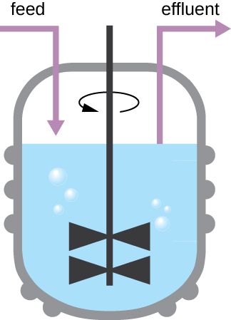
Sustaining Microbial Growth

The growth pattern shown in Figure \(\PageIndex{4}\) takes place in a closed environment; nutrients are not added and waste and dead cells are not removed. In many cases, though, it is advantageous to maintain cells in the logarithmic phase of growth. One example is in industries that harvest microbial products. A chemostat (Figure \(\PageIndex{6}\)) is used to maintain a continuous culture in which nutrients are supplied at a steady rate. A controlled amount of air is mixed in for aerobic processes. Bacterial suspension is removed at the same rate as nutrients flow in to maintain an optimal growth environment.

Figure \(\PageIndex{6}\): A chemostat is a culture vessel fitted with an opening to add nutrients (feed) and an outlet to remove contents (effluent), effectively diluting toxic wastes and dead cells. The addition and removal of fluids is adjusted to maintain the culture in the logarithmic phase of growth. If aerobic bacteria are grown, suitable oxygen levels are maintained.

Key Concepts and Summary

• Cells in a closed system follow a pattern of growth with four phases: lag, logarithmic (exponential), stationary, and death.