19.1C: Hardy-Weinberg Principle of Equilibrium
- Page ID
- 13480
\( \newcommand{\vecs}[1]{\overset { \scriptstyle \rightharpoonup} {\mathbf{#1}} } \)
\( \newcommand{\vecd}[1]{\overset{-\!-\!\rightharpoonup}{\vphantom{a}\smash {#1}}} \)
\( \newcommand{\id}{\mathrm{id}}\) \( \newcommand{\Span}{\mathrm{span}}\)
( \newcommand{\kernel}{\mathrm{null}\,}\) \( \newcommand{\range}{\mathrm{range}\,}\)
\( \newcommand{\RealPart}{\mathrm{Re}}\) \( \newcommand{\ImaginaryPart}{\mathrm{Im}}\)
\( \newcommand{\Argument}{\mathrm{Arg}}\) \( \newcommand{\norm}[1]{\| #1 \|}\)
\( \newcommand{\inner}[2]{\langle #1, #2 \rangle}\)
\( \newcommand{\Span}{\mathrm{span}}\)
\( \newcommand{\id}{\mathrm{id}}\)
\( \newcommand{\Span}{\mathrm{span}}\)
\( \newcommand{\kernel}{\mathrm{null}\,}\)
\( \newcommand{\range}{\mathrm{range}\,}\)
\( \newcommand{\RealPart}{\mathrm{Re}}\)
\( \newcommand{\ImaginaryPart}{\mathrm{Im}}\)
\( \newcommand{\Argument}{\mathrm{Arg}}\)
\( \newcommand{\norm}[1]{\| #1 \|}\)
\( \newcommand{\inner}[2]{\langle #1, #2 \rangle}\)
\( \newcommand{\Span}{\mathrm{span}}\) \( \newcommand{\AA}{\unicode[.8,0]{x212B}}\)
\( \newcommand{\vectorA}[1]{\vec{#1}} % arrow\)
\( \newcommand{\vectorAt}[1]{\vec{\text{#1}}} % arrow\)
\( \newcommand{\vectorB}[1]{\overset { \scriptstyle \rightharpoonup} {\mathbf{#1}} } \)
\( \newcommand{\vectorC}[1]{\textbf{#1}} \)
\( \newcommand{\vectorD}[1]{\overrightarrow{#1}} \)
\( \newcommand{\vectorDt}[1]{\overrightarrow{\text{#1}}} \)
\( \newcommand{\vectE}[1]{\overset{-\!-\!\rightharpoonup}{\vphantom{a}\smash{\mathbf {#1}}}} \)
\( \newcommand{\vecs}[1]{\overset { \scriptstyle \rightharpoonup} {\mathbf{#1}} } \)
\( \newcommand{\vecd}[1]{\overset{-\!-\!\rightharpoonup}{\vphantom{a}\smash {#1}}} \)
\(\newcommand{\avec}{\mathbf a}\) \(\newcommand{\bvec}{\mathbf b}\) \(\newcommand{\cvec}{\mathbf c}\) \(\newcommand{\dvec}{\mathbf d}\) \(\newcommand{\dtil}{\widetilde{\mathbf d}}\) \(\newcommand{\evec}{\mathbf e}\) \(\newcommand{\fvec}{\mathbf f}\) \(\newcommand{\nvec}{\mathbf n}\) \(\newcommand{\pvec}{\mathbf p}\) \(\newcommand{\qvec}{\mathbf q}\) \(\newcommand{\svec}{\mathbf s}\) \(\newcommand{\tvec}{\mathbf t}\) \(\newcommand{\uvec}{\mathbf u}\) \(\newcommand{\vvec}{\mathbf v}\) \(\newcommand{\wvec}{\mathbf w}\) \(\newcommand{\xvec}{\mathbf x}\) \(\newcommand{\yvec}{\mathbf y}\) \(\newcommand{\zvec}{\mathbf z}\) \(\newcommand{\rvec}{\mathbf r}\) \(\newcommand{\mvec}{\mathbf m}\) \(\newcommand{\zerovec}{\mathbf 0}\) \(\newcommand{\onevec}{\mathbf 1}\) \(\newcommand{\real}{\mathbb R}\) \(\newcommand{\twovec}[2]{\left[\begin{array}{r}#1 \\ #2 \end{array}\right]}\) \(\newcommand{\ctwovec}[2]{\left[\begin{array}{c}#1 \\ #2 \end{array}\right]}\) \(\newcommand{\threevec}[3]{\left[\begin{array}{r}#1 \\ #2 \\ #3 \end{array}\right]}\) \(\newcommand{\cthreevec}[3]{\left[\begin{array}{c}#1 \\ #2 \\ #3 \end{array}\right]}\) \(\newcommand{\fourvec}[4]{\left[\begin{array}{r}#1 \\ #2 \\ #3 \\ #4 \end{array}\right]}\) \(\newcommand{\cfourvec}[4]{\left[\begin{array}{c}#1 \\ #2 \\ #3 \\ #4 \end{array}\right]}\) \(\newcommand{\fivevec}[5]{\left[\begin{array}{r}#1 \\ #2 \\ #3 \\ #4 \\ #5 \\ \end{array}\right]}\) \(\newcommand{\cfivevec}[5]{\left[\begin{array}{c}#1 \\ #2 \\ #3 \\ #4 \\ #5 \\ \end{array}\right]}\) \(\newcommand{\mattwo}[4]{\left[\begin{array}{rr}#1 \amp #2 \\ #3 \amp #4 \\ \end{array}\right]}\) \(\newcommand{\laspan}[1]{\text{Span}\{#1\}}\) \(\newcommand{\bcal}{\cal B}\) \(\newcommand{\ccal}{\cal C}\) \(\newcommand{\scal}{\cal S}\) \(\newcommand{\wcal}{\cal W}\) \(\newcommand{\ecal}{\cal E}\) \(\newcommand{\coords}[2]{\left\{#1\right\}_{#2}}\) \(\newcommand{\gray}[1]{\color{gray}{#1}}\) \(\newcommand{\lgray}[1]{\color{lightgray}{#1}}\) \(\newcommand{\rank}{\operatorname{rank}}\) \(\newcommand{\row}{\text{Row}}\) \(\newcommand{\col}{\text{Col}}\) \(\renewcommand{\row}{\text{Row}}\) \(\newcommand{\nul}{\text{Nul}}\) \(\newcommand{\var}{\text{Var}}\) \(\newcommand{\corr}{\text{corr}}\) \(\newcommand{\len}[1]{\left|#1\right|}\) \(\newcommand{\bbar}{\overline{\bvec}}\) \(\newcommand{\bhat}{\widehat{\bvec}}\) \(\newcommand{\bperp}{\bvec^\perp}\) \(\newcommand{\xhat}{\widehat{\xvec}}\) \(\newcommand{\vhat}{\widehat{\vvec}}\) \(\newcommand{\uhat}{\widehat{\uvec}}\) \(\newcommand{\what}{\widehat{\wvec}}\) \(\newcommand{\Sighat}{\widehat{\Sigma}}\) \(\newcommand{\lt}{<}\) \(\newcommand{\gt}{>}\) \(\newcommand{\amp}{&}\) \(\definecolor{fillinmathshade}{gray}{0.9}\)- Use the Hardy Weinberg equation to calculate allelic and genotypic frequencies in a population
The Hardy-Weinberg principle states that a population’s allele and genotype frequencies will remain constant in the absence of evolutionary mechanisms. Ultimately, the Hardy-Weinberg principle models a population without evolution under the following conditions:
- no mutations
- no immigration/emigration
- no natural selection
- no sexual selection
- a large population
Although no real-world population can satisfy all of these conditions, the principle still offers a useful model for population analysis.
Hardy-Weinberg Equations and Analysis
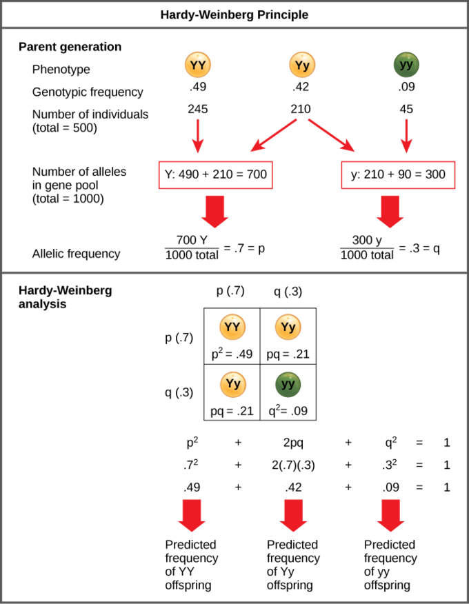
According to the Hardy-Weinberg principle, the variable p often represents the frequency of a particular allele, usually a dominant one. For example, assume that p represents the frequency of the dominant allele, Y, for yellow pea pods. The variable q represents the frequency of the recessive allele, y, for green pea pods. If p and q are the only two possible alleles for this characteristic, then the sum of the frequencies must add up to 1, or 100 percent. We can also write this as p + q = 1.If the frequency of the Y allele in the population is 0.6, then we know that the frequency of the y allele is 0.4.
From the Hardy-Weinberg principle and the known allele frequencies, we can also infer the frequencies of the genotypes. Since each individual carries two alleles per gene (Y or y), we can predict the frequencies of these genotypes with a chi square. If two alleles are drawn at random from the gene pool, we can determine the probability of each genotype.
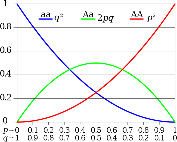
In the example, our three genotype possibilities are: pp (YY), producing yellow peas; pq (Yy), also yellow; or qq (yy), producing green peas. The frequency of homozygous pp individuals is p2; the frequency of hereozygous pq individuals is 2pq; and the frequency of homozygous qq individuals is q2. If p and q are the only two possible alleles for a given trait in the population, these genotypes frequencies will sum to one: p2 + 2pq + q2 = 1.

In our example, the possible genotypes are homozygous dominant (YY), heterozygous (Yy), and homozygous recessive (yy). If we can only observe the phenotypes in the population, then we know only the recessive phenotype (yy). For example, in a garden of 100 pea plants, 86 might have yellow peas and 16 have green peas. We do not know how many are homozygous dominant (Yy) or heterozygous (Yy), but we do know that 16 of them are homozygous recessive (yy).
Therefore, by knowing the recessive phenotype and, thereby, the frequency of that genotype (16 out of 100 individuals or 0.16), we can calculate the number of other genotypes. If q2 represents the frequency of homozygous recessive plants, then q2 = 0.16. Therefore, q = 0.4.Because p + q = 1, then 1 – 0.4 = p, and we know that p = 0.6. The frequency of homozygous dominant plants (p2) is (0.6)2 = 0.36. Out of 100 individuals, there are 36 homozygous dominant (YY) plants. The frequency of heterozygous plants (2pq) is 2(0.6)(0.4) = 0.48. Therefore, 48 out of 100 plants are heterozygous yellow (Yy).

Applications of Hardy-Weinberg
The genetic variation of natural populations is constantly changing from genetic drift, mutation, migration, and natural and sexual selection. The Hardy-Weinberg principle gives scientists a mathematical baseline of a non-evolving population to which they can compare evolving populations. If scientists record allele frequencies over time and then calculate the expected frequencies based on Hardy-Weinberg values, the scientists can hypothesize the mechanisms driving the population’s evolution.
Key Points
- The Hardy-Weinberg principle assumes that in a given population, the population is large and is not experiencing mutation, migration, natural selection, or sexual selection.
- The frequency of alleles in a population can be represented by p + q = 1, with p equal to the frequency of the dominant allele and q equal to the frequency of the recessive allele.
- The frequency of genotypes in a population can be represented by p2+2pq+q2= 1, with p2 equal to the frequency of the homozygous dominant genotype, 2pq equal to the frequency of the heterozygous genotype, and q2 equal to the frequency of the recessive genotype.
- The frequency of alleles can be estimated by calculating the frequency of the recessive genotype, then calculating the square root of that frequency in order to determine the frequency of the recessive allele.
Key Terms
- genotype: the combination of alleles, situated on corresponding chromosomes, that determines a specific trait of an individual, such as “Aa” or “aa”
- phenotype: the appearance of an organism based on a multifactorial combination of genetic traits and environmental factors, especially used in pedigrees
Contributions and Attributions
- OpenStax College, Biology. October 16, 2013. Provided by: OpenStax CNX. Located at: http://cnx.org/content/m44575/latest...ol11448/latest. License: CC BY: Attribution
- Evolution. Provided by: Wikipedia. Located at: en.Wikipedia.org/wiki/Evolution%23Mechanisms. License: CC BY-SA: Attribution-ShareAlike
- gene flow. Provided by: Wikipedia. Located at: en.Wikipedia.org/wiki/gene%20flow. License: CC BY-SA: Attribution-ShareAlike
- Boundless. Provided by: Boundless Learning. Located at: www.boundless.com//biology/de...ic-hitchhiking. License: CC BY-SA: Attribution-ShareAlike
- fitness. Provided by: Wikipedia. Located at: en.Wikipedia.org/wiki/fitness. License: CC BY-SA: Attribution-ShareAlike
- mutation. Provided by: Wiktionary. Located at: en.wiktionary.org/wiki/mutation. License: CC BY-SA: Attribution-ShareAlike
- Natural Selection. Provided by: Wikipedia. Located at: en.Wikipedia.org/wiki/Natural_selection. License: CC BY-SA: Attribution-ShareAlike
- genetic drift. Provided by: Wiktionary. Located at: en.wiktionary.org/wiki/genetic_drift. License: CC BY-SA: Attribution-ShareAlike
- natural selection. Provided by: Wiktionary. Located at: en.wiktionary.org/wiki/natural_selection. License: CC BY-SA: Attribution-ShareAlike
- OpenStax College, Introduction. October 16, 2013. Provided by: OpenStax CNX. Located at: http://cnx.org/content/m44575/latest...e_19_00_01.jpg. License: CC BY: Attribution
- Mutation and selection diagram. Provided by: Wikipedia. Located at: en.Wikipedia.org/wiki/File:Mu...on_diagram.svg. License: CC BY-SA: Attribution-ShareAlike
- Random sampling genetic drift. Provided by: Wikipedia. Located at: en.Wikipedia.org/wiki/File:Ra...etic_drift.svg. License: CC BY-SA: Attribution-ShareAlike
- OpenStax College, Biology. October 16, 2013. Provided by: OpenStax CNX. Located at: http://cnx.org/content/m44582/latest...ol11448/latest. License: CC BY: Attribution
- allele. Provided by: Wiktionary. Located at: en.wiktionary.org/wiki/allele. License: CC BY-SA: Attribution-ShareAlike
- Population Genetics. Provided by: Wikpedia. Located at: en.Wikipedia.org/wiki/Population_genetics. License: CC BY-SA: Attribution-ShareAlike
- founder effect. Provided by: Wiktionary. Located at: en.wiktionary.org/wiki/founder_effect. License: CC BY-SA: Attribution-ShareAlike
- gene pool. Provided by: Wiktionary. Located at: en.wiktionary.org/wiki/gene_pool. License: CC BY-SA: Attribution-ShareAlike
- OpenStax College, Introduction. October 16, 2013. Provided by: OpenStax CNX. Located at: http://cnx.org/content/m44575/latest...e_19_00_01.jpg. License: CC BY: Attribution
- Mutation and selection diagram. Provided by: Wikipedia. Located at: en.Wikipedia.org/wiki/File:Mu...on_diagram.svg. License: CC BY-SA: Attribution-ShareAlike
- Random sampling genetic drift. Provided by: Wikipedia. Located at: en.Wikipedia.org/wiki/File:Ra...etic_drift.svg. License: CC BY-SA: Attribution-ShareAlike
- ABO Blood type. Provided by: Wikimedia. Located at: en.Wikipedia.org/wiki/ABO_blo...blood_type.svg. License: Public Domain: No Known Copyright
- Founder effect. Provided by: Wikipedia. Located at: en.Wikipedia.org/wiki/File:Founder_effect.png. License: Public Domain: No Known Copyright
- OpenStax College, Biology. October 16, 2013. Provided by: OpenStax CNX. Located at: http://cnx.org/content/m44582/latest...ol11448/latest. License: CC BY: Attribution
- genotype. Provided by: Wiktionary. Located at: en.wiktionary.org/wiki/genotype. License: CC BY-SA: Attribution-ShareAlike
- phenotype. Provided by: Wiktionary. Located at: en.wiktionary.org/wiki/phenotype. License: CC BY-SA: Attribution-ShareAlike
- OpenStax College, Introduction. October 16, 2013. Provided by: OpenStax CNX. Located at: http://cnx.org/content/m44575/latest...e_19_00_01.jpg. License: CC BY: Attribution
- Mutation and selection diagram. Provided by: Wikipedia. Located at: en.Wikipedia.org/wiki/File:Mu...on_diagram.svg. License: CC BY-SA: Attribution-ShareAlike
- Random sampling genetic drift. Provided by: Wikipedia. Located at: en.Wikipedia.org/wiki/File:Ra...etic_drift.svg. License: CC BY-SA: Attribution-ShareAlike
- ABO Blood type. Provided by: Wikimedia. Located at: en.Wikipedia.org/wiki/ABO_blo...blood_type.svg. License: Public Domain: No Known Copyright
- Founder effect. Provided by: Wikipedia. Located at: en.Wikipedia.org/wiki/File:Founder_effect.png. License: Public Domain: No Known Copyright
- OpenStax College, Population Evolution. October 16, 2013. Provided by: OpenStax CNX. Located at: http://cnx.org/content/m44582/latest...e_19_01_01.png. License: CC BY: Attribution
- Hardy-Weinberg. Provided by: Wikimedia. Located at: en.Wikipedia.org/wiki/Hardy-W...y-Weinberg.svg. License: CC BY-SA: Attribution-ShareAlike


