
2: Allele and Genotype Frequencies
- Page ID
- 96506

\( \newcommand{\vecs}[1]{\overset { \scriptstyle \rightharpoonup} {\mathbf{#1}} } \)
\( \newcommand{\vecd}[1]{\overset{-\!-\!\rightharpoonup}{\vphantom{a}\smash {#1}}} \)
\( \newcommand{\dsum}{\displaystyle\sum\limits} \)
\( \newcommand{\dint}{\displaystyle\int\limits} \)
\( \newcommand{\dlim}{\displaystyle\lim\limits} \)
\( \newcommand{\id}{\mathrm{id}}\) \( \newcommand{\Span}{\mathrm{span}}\)
( \newcommand{\kernel}{\mathrm{null}\,}\) \( \newcommand{\range}{\mathrm{range}\,}\)
\( \newcommand{\RealPart}{\mathrm{Re}}\) \( \newcommand{\ImaginaryPart}{\mathrm{Im}}\)
\( \newcommand{\Argument}{\mathrm{Arg}}\) \( \newcommand{\norm}[1]{\| #1 \|}\)
\( \newcommand{\inner}[2]{\langle #1, #2 \rangle}\)
\( \newcommand{\Span}{\mathrm{span}}\)
\( \newcommand{\id}{\mathrm{id}}\)
\( \newcommand{\Span}{\mathrm{span}}\)
\( \newcommand{\kernel}{\mathrm{null}\,}\)
\( \newcommand{\range}{\mathrm{range}\,}\)
\( \newcommand{\RealPart}{\mathrm{Re}}\)
\( \newcommand{\ImaginaryPart}{\mathrm{Im}}\)
\( \newcommand{\Argument}{\mathrm{Arg}}\)
\( \newcommand{\norm}[1]{\| #1 \|}\)
\( \newcommand{\inner}[2]{\langle #1, #2 \rangle}\)
\( \newcommand{\Span}{\mathrm{span}}\) \( \newcommand{\AA}{\unicode[.8,0]{x212B}}\)
\( \newcommand{\vectorA}[1]{\vec{#1}} % arrow\)
\( \newcommand{\vectorAt}[1]{\vec{\text{#1}}} % arrow\)
\( \newcommand{\vectorB}[1]{\overset { \scriptstyle \rightharpoonup} {\mathbf{#1}} } \)
\( \newcommand{\vectorC}[1]{\textbf{#1}} \)
\( \newcommand{\vectorD}[1]{\overrightarrow{#1}} \)
\( \newcommand{\vectorDt}[1]{\overrightarrow{\text{#1}}} \)
\( \newcommand{\vectE}[1]{\overset{-\!-\!\rightharpoonup}{\vphantom{a}\smash{\mathbf {#1}}}} \)
\( \newcommand{\vecs}[1]{\overset { \scriptstyle \rightharpoonup} {\mathbf{#1}} } \)
\(\newcommand{\longvect}{\overrightarrow}\)
\( \newcommand{\vecd}[1]{\overset{-\!-\!\rightharpoonup}{\vphantom{a}\smash {#1}}} \)
\(\newcommand{\avec}{\mathbf a}\) \(\newcommand{\bvec}{\mathbf b}\) \(\newcommand{\cvec}{\mathbf c}\) \(\newcommand{\dvec}{\mathbf d}\) \(\newcommand{\dtil}{\widetilde{\mathbf d}}\) \(\newcommand{\evec}{\mathbf e}\) \(\newcommand{\fvec}{\mathbf f}\) \(\newcommand{\nvec}{\mathbf n}\) \(\newcommand{\pvec}{\mathbf p}\) \(\newcommand{\qvec}{\mathbf q}\) \(\newcommand{\svec}{\mathbf s}\) \(\newcommand{\tvec}{\mathbf t}\) \(\newcommand{\uvec}{\mathbf u}\) \(\newcommand{\vvec}{\mathbf v}\) \(\newcommand{\wvec}{\mathbf w}\) \(\newcommand{\xvec}{\mathbf x}\) \(\newcommand{\yvec}{\mathbf y}\) \(\newcommand{\zvec}{\mathbf z}\) \(\newcommand{\rvec}{\mathbf r}\) \(\newcommand{\mvec}{\mathbf m}\) \(\newcommand{\zerovec}{\mathbf 0}\) \(\newcommand{\onevec}{\mathbf 1}\) \(\newcommand{\real}{\mathbb R}\) \(\newcommand{\twovec}[2]{\left[\begin{array}{r}#1 \\ #2 \end{array}\right]}\) \(\newcommand{\ctwovec}[2]{\left[\begin{array}{c}#1 \\ #2 \end{array}\right]}\) \(\newcommand{\threevec}[3]{\left[\begin{array}{r}#1 \\ #2 \\ #3 \end{array}\right]}\) \(\newcommand{\cthreevec}[3]{\left[\begin{array}{c}#1 \\ #2 \\ #3 \end{array}\right]}\) \(\newcommand{\fourvec}[4]{\left[\begin{array}{r}#1 \\ #2 \\ #3 \\ #4 \end{array}\right]}\) \(\newcommand{\cfourvec}[4]{\left[\begin{array}{c}#1 \\ #2 \\ #3 \\ #4 \end{array}\right]}\) \(\newcommand{\fivevec}[5]{\left[\begin{array}{r}#1 \\ #2 \\ #3 \\ #4 \\ #5 \\ \end{array}\right]}\) \(\newcommand{\cfivevec}[5]{\left[\begin{array}{c}#1 \\ #2 \\ #3 \\ #4 \\ #5 \\ \end{array}\right]}\) \(\newcommand{\mattwo}[4]{\left[\begin{array}{rr}#1 \amp #2 \\ #3 \amp #4 \\ \end{array}\right]}\) \(\newcommand{\laspan}[1]{\text{Span}\{#1\}}\) \(\newcommand{\bcal}{\cal B}\) \(\newcommand{\ccal}{\cal C}\) \(\newcommand{\scal}{\cal S}\) \(\newcommand{\wcal}{\cal W}\) \(\newcommand{\ecal}{\cal E}\) \(\newcommand{\coords}[2]{\left\{#1\right\}_{#2}}\) \(\newcommand{\gray}[1]{\color{gray}{#1}}\) \(\newcommand{\lgray}[1]{\color{lightgray}{#1}}\) \(\newcommand{\rank}{\operatorname{rank}}\) \(\newcommand{\row}{\text{Row}}\) \(\newcommand{\col}{\text{Col}}\) \(\renewcommand{\row}{\text{Row}}\) \(\newcommand{\nul}{\text{Nul}}\) \(\newcommand{\var}{\text{Var}}\) \(\newcommand{\corr}{\text{corr}}\) \(\newcommand{\len}[1]{\left|#1\right|}\) \(\newcommand{\bbar}{\overline{\bvec}}\) \(\newcommand{\bhat}{\widehat{\bvec}}\) \(\newcommand{\bperp}{\bvec^\perp}\) \(\newcommand{\xhat}{\widehat{\xvec}}\) \(\newcommand{\vhat}{\widehat{\vvec}}\) \(\newcommand{\uhat}{\widehat{\uvec}}\) \(\newcommand{\what}{\widehat{\wvec}}\) \(\newcommand{\Sighat}{\widehat{\Sigma}}\) \(\newcommand{\lt}{<}\) \(\newcommand{\gt}{>}\) \(\newcommand{\amp}{&}\) \(\definecolor{fillinmathshade}{gray}{0.9}\)In this chapter we will work through how the basics of Mendelian genetics play out at the population level in sexually reproducing organisms.
Loci and alleles are the basic currency of population genetics–and indeed of genetics. A locus may be an entire gene, or a single nucleotide base pair such as A-T. At each locus, there may be multiple genetic variants segregating in the population—these different genetic variants are known as alleles. If all individuals in the population carry the same allele, we say that the locus is monomorphic; at this locus there is no genetic variability in the population. If there are multiple alleles in the population at a locus, we say that this locus is polymorphic (this is sometimes referred to as a segregating site).
|
pos. |
con. |
a |
b |
c |
d |
e |
f |
g |
h |
i |
j |
k |
l |
a |
b |
c |
d |
e |
f |
a |
b |
c |
d |
e |
f |
g |
h |
i |
j |
k |
l |
NS/S |
||
|---|---|---|---|---|---|---|---|---|---|---|---|---|---|---|---|---|---|---|---|---|---|---|---|---|---|---|---|---|---|---|---|---|---|---|
|
781 |
G |
T |
T |
T |
T |
T |
T |
T |
T |
T |
T |
T |
T |
- |
- |
- |
- |
- |
- |
- |
- |
- |
- |
- |
- |
- |
- |
- |
- |
- |
- |
NS |
||
|
789 |
T |
- |
- |
- |
- |
- |
- |
- |
- |
- |
- |
- |
- |
- |
- |
- |
- |
- |
- |
C |
C |
C |
C |
C |
C |
C |
C |
C |
C |
C |
C |
S |
||
|
808 |
A |
- |
- |
- |
- |
- |
- |
- |
- |
- |
- |
- |
- |
- |
- |
- |
- |
- |
- |
G |
G |
G |
G |
G |
G |
G |
G |
G |
G |
G |
G |
NS |
||
|
816 |
G |
T |
T |
T |
T |
- |
- |
- |
- |
- |
- |
- |
T |
T |
T |
T |
T |
T |
T |
- |
- |
- |
- |
- |
- |
- |
- |
- |
- |
- |
- |
S |
||
|
834 |
T |
- |
- |
- |
- |
- |
- |
- |
- |
- |
- |
- |
- |
C |
C |
- |
- |
- |
C |
- |
- |
- |
- |
- |
- |
- |
- |
- |
- |
- |
- |
S |
||
|
859 |
C |
- |
- |
- |
- |
- |
- |
- |
- |
- |
- |
- |
- |
- |
- |
- |
- |
- |
- |
G |
G |
G |
G |
G |
G |
G |
G |
G |
G |
G |
G |
NS |
||
|
867 |
C |
- |
- |
- |
- |
- |
- |
- |
- |
- |
- |
- |
- |
- |
- |
- |
- |
- |
- |
G |
G |
G |
G |
G |
A |
G |
G |
G |
G |
G |
G |
S |
||
|
870 |
C |
T |
T |
T |
T |
T |
T |
T |
T |
T |
T |
T |
T |
- |
- |
- |
- |
- |
- |
- |
- |
- |
- |
- |
- |
- |
- |
- |
- |
- |
- |
S |
||
|
950 |
G |
- |
- |
- |
- |
- |
- |
- |
- |
- |
- |
- |
- |
- |
A |
- |
- |
- |
- |
- |
- |
- |
- |
- |
- |
- |
- |
- |
- |
- |
- |
S |
||
|
974 |
G |
- |
- |
- |
- |
- |
- |
- |
- |
- |
- |
- |
- |
T |
- |
T |
T |
T |
T |
- |
- |
- |
- |
- |
- |
- |
- |
- |
- |
- |
- |
S |
||
|
983 |
T |
- |
- |
- |
- |
- |
- |
- |
- |
- |
- |
- |
- |
- |
- |
- |
- |
- |
- |
C |
C |
C |
C |
C |
C |
C |
C |
C |
C |
C |
C |
S |
||
|
1019 |
C |
- |
- |
- |
- |
- |
- |
- |
- |
- |
- |
- |
- |
- |
- |
- |
- |
- |
- |
- |
- |
- |
- |
A |
- |
- |
- |
- |
- |
- |
- |
S |
||
|
1031 |
C |
- |
- |
- |
- |
- |
- |
- |
- |
- |
- |
- |
- |
- |
- |
- |
- |
- |
- |
- |
- |
- |
- |
- |
- |
- |
- |
A |
- |
- |
- |
S |
||
|
1034 |
T |
- |
- |
- |
- |
- |
- |
- |
- |
- |
- |
- |
- |
- |
- |
- |
- |
- |
- |
C |
C |
C |
C |
C |
- |
- |
C |
- |
C |
C |
S |
|||
|
1043 |
C |
- |
- |
- |
- |
- |
- |
- |
- |
- |
- |
- |
- |
- |
- |
- |
- |
- |
- |
- |
- |
- |
- |
A |
- |
- |
- |
- |
- |
- |
- |
S |
||
|
1068 |
C |
T |
T |
- |
- |
- |
- |
- |
- |
- |
- |
- |
- |
- |
- |
- |
- |
- |
- |
- |
- |
- |
- |
- |
- |
- |
- |
- |
- |
- |
- |
S |
||
|
1089 |
C |
- |
- |
- |
- |
- |
- |
- |
- |
- |
- |
- |
- |
A |
A |
A |
A |
A |
A |
- |
- |
- |
- |
- |
- |
- |
- |
- |
- |
- |
- |
NS |
||
|
1101 |
G |
- |
- |
- |
- |
- |
- |
- |
- |
- |
- |
- |
- |
- |
- |
- |
- |
- |
- |
A |
A |
A |
A |
A |
A |
A |
A |
A |
A |
A |
A |
NS |
||
|
1127 |
T |
- |
- |
- |
- |
- |
- |
- |
- |
- |
- |
- |
- |
- |
- |
- |
- |
- |
- |
C |
C |
C |
C |
C |
C |
C |
C |
C |
C |
C |
C |
S |
||
|
1131 |
C |
- |
- |
- |
- |
- |
- |
- |
- |
- |
- |
- |
- |
- |
- |
- |
- |
- |
- |
- |
- |
- |
- |
T |
- |
- |
- |
- |
- |
- |
- |
S |
||
|
1160 |
T |
- |
- |
- |
- |
- |
- |
- |
- |
- |
- |
- |
- |
- |
- |
- |
- |
- |
- |
C |
C |
C |
C |
C |
C |
C |
C |
C |
C |
C |
C |
S |
Table \(\PageIndex{1}\) shows a small stretch of orthologous sequence for the ADH locus from samples from Drosophila melanogaster, D. simulans, and D. yakuba. D. melanogaster and D. simulans are sister species and D. yakuba is a close outgroup to the two. Each column represents a single haplotype from an individual (the individuals are diploid but were inbred so they’re homozygous for their haplotype). Only sites that differ among individuals of the three species are shown. Site \(834\) is an example of a polymorphism; some D. simulans individuals carry a \(C\) allele while others have a \(T\). Fixed differences are sites that differ between the species but are monomorphic within the species. Site \(781\) is an example of a fixed difference between D. melanogaster and the other two species.
We can also annotate the alleles and loci in various ways. For example, position \(781\) is a non-synonymous fixed difference. We call the less common allele at a polymorphism the minor allele and the common allele the major allele, e.g. at site \(1068\) the \(T\) allele is the minor allele in D. melanogaster. We call the more evolutionarily recent of the two alleles the derived allele and the older of the two the ancestral allele. We infer that the \(T\) allele at site 1068 is the derived allele because the \(C\) is found in both other species, suggesting that the \(T\) allele arose via a \(C \rightarrow T\) mutation.
- How many segregating sites does the sample from D. simulans have in the ADH gene?
- How many fixed differences are there between D. melanogaster and D. yakuba?
Allele frequencies
Allele frequencies are a central unit of population genetics analysis, but from diploid individuals we only get to observe genotype counts. Our first task then is to calculate allele frequencies from genotype counts. Consider a diploid autosomal locus segregating for two alleles (\(A_1\) and \(A_2\)). We’ll use these arbitrary labels for our alleles, merely to keep this general. Let \(N_{11}\) and \(N_{12}\) be the number of \(A_1A_1\) homozygotes and \(A_1A_2\) heterozygotes, respectively. Moreover, let \(N\) be the total number of diploid individuals in the population. We can then define the relative frequencies of \(A_1A_1\) and \(A_1A_2\) genotypes as \(f_{11} = N_{11}/N\) and \(f_{12} = N_{12}/N\), respectively. The frequency of allele \(A_1\) in the population is then given by
\[p = \frac{2 N_{11} + N_{12}}{2N} = f_{11} + \frac{1}{2} f_{12}. \nonumber\]
Note that this follows directly from how we count alleles given individuals’ genotypes, and holds independently of Hardy–Weinberg proportions and equilibrium (discussed below). The frequency of the alternate allele (\(A_2\)) is then just \(q=1-p\).
Measures of genetic variability
Nucleotide diversity (\(\pi\)) - One common measure of genetic diversity is the average number of single nucleotide differences between haplotypes chosen at random from a sample. This is called nucleotide diversity and is often denoted by \(\pi\). For example, we can calculate \(\pi\) for our ADH locus from Table \ref{Table:ADH} above: we have 6 sequences from D. simulans (a-f), there’s a total of 15 ways of pairing these sequences, and
\[\pi=\frac{1}{15} \big( (2 + 1 + 1 + 1 + 0 ) + (3 + 3 + 3 + 2 ) +(0 + 0 + 1) + (0 + 1) + (1) \big)=1.2\overline{6}\]
where the first bracketed term gives the pairwise differences between a and b-f, the second bracketed term the differences between b and c-f and so on.
Our \(\pi\) measure will depend on the length of sequence it is calculated for. Therefore, \(\pi\) is usually normalized by the length of sequence, to be a per site (or per base) measure. For example, our ADH sequence covers \(397\)bp of DNA and so \(\pi = 1.2\overline{6}/397=0.0032\) per site in D. simulans for this region. Note that we could also calculate \(\pi\) per synonymous site (or non-synonymous). For synonymous site \(\pi\), we would count up number of synonymous differences between our pairs of sequences, and then divide by the total number of sites where a synonymous change could have occurred.Technically we would need to divide by the total number of possible point mutations that would result in a synonymous change; this is because some mutational changes at a particular nucleotide will result in a non-synonymous or synonymous change depending on the base-pair change.
Number of segregating sites
Another measure of genetic variability is the total number of sites that are polymorphic (segregating) in our sample. One issue is that the number of segregating sites will grow as we sequence more individuals (unlike \(\pi\)). Later in the course, we’ll talk about how to standardize the number of segregating sites for the number of individuals sequenced (see \ref{watterson_theta}).
The frequency spectrum
We also often want to compile information about the frequency of alleles across sites. We call alleles that are found once in a sample singletons, alleles that are found twice in a sample doubletons, and so on. We count up the number of loci where an allele is found \(i\) times out of \(n\), e.g. how many singletons are there in the sample, and this is called the frequency spectrum. We’ll want to do this in some consistent manner, such as calculating the frequency spectrum of the minor allele or the derived allele.
How many minor-allele singletons are there in D. simulans in the ADH region? [Defining minor allele just within D. simulans.]
Levels of genetic variability across species
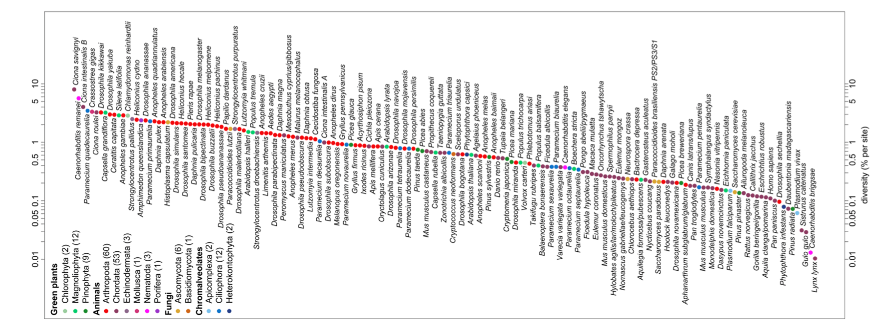
Two observations have puzzled population geneticists since the inception of molecular population genetics. The first is the relatively high level of genetic variation observed in most obligately sexual species. This first observation, in part, drove the development of the Neutral theory of molecular evolution, the idea that much of this molecular polymorphism may simply reflect a balance between genetic drift and mutation. The second observation is the relatively narrow range of polymorphism across species with vastly different census sizes. This observation represented a puzzle as the Neutral theory predicts that levels of genetic diversity should scale with population size. Much effort in theoretical and empirical population genetics has been devoted to trying to reconcile models with these various observations. We’ll return to discuss these ideas throughout our course.
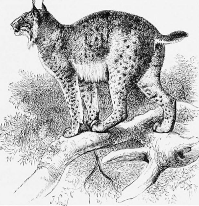
The first observations of molecular genetic diversity within natural populations were made from surveys of allozyme data, but we can revisit these general patterns with modern data. For example, Leffler et al. (2012) compiled data on levels of within-population, autosomal nucleotide diversity (π) for 167 species across 14 phyla from non-coding and synonymous sites (Figure 2.3). The species with the lowest levels of π in their survey was Lynx, with π = 0.01%, i.e. only 1/10000 bases differed between two sequences. In contrast, some of the highest levels of diversity were found in Ciona savignyi, Sea Squirts, where a remarkable 1/12 bases differ between pairs of sequences. This 800-fold range of diversity seems impressive, but census population sizes have a much larger range.
Hardy–Weinberg proportions
Imagine a population mating at random with respect to genotypes, i.e. no inbreeding, no assortative mating, no population structure, and no sex differences in allele frequencies. The frequency of allele \(A_1\) in the population at the time of reproduction is \(p\). An \(A_1A_1\) genotype is made by reaching out into our population and independently drawing two \(A_1\) allele gametes to form a zygote. Therefore, the probability that an individual is an \(A_1A_1\) homozygote is \(p^2\). This probability is also the expected frequencies of the \(A_1A_1\) homozygote in the population. The expected frequency of the three possible genotypes are
| \(f_{11}\) | \(f_{12}\) | \(f_{22}\) |
|---|---|---|
| \(p^2\) | \(2pq\) | \(q^2\) |
i.e. their Hardy-Weinberg expectations . Note that we only need to assume random mating with respect to our focal allele in order for these expected frequencies to hold in the zygotes forming the next generation. Evolutionary forces, such as selection, change allele frequencies within generations, but do not change this expectation for new zygotes, as long as \(p\) is the frequency of the \(A_1\) allele in the population at the time when gametes fuse. We only need the assumptions of no migration, selection, and mutation in order for these Hardy-Weinberg expectations of genotypes to represent a long term equilibrium.
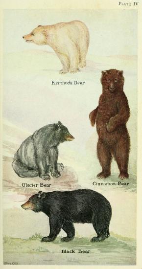
On the coastal islands of British Columbia there is a subspecies of black bear (Ursus americanus kermodei, Kermode’s bear). Many members of this black bear subspecies are white; they’re sometimes called spirit bears. These bears aren’t hybrids with polar bears, nor are they albinos. They are homozygotes for a recessive change at the MC1R gene. Individuals who are \(GG\) at this SNP are white, while \(AA\) and \(AG\) individuals are black.
Below are the genotype counts for the MC1R polymorphism in a sample of bears from British Columbia’s island populations from .
| \(AA\) | \(AG\) | \(GG\) |
|---|---|---|
| 42 | 24 | 21 |
What are the expected frequencies of the three genotypes under HW?
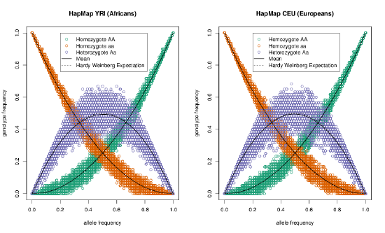
See Figure \ref{fig:HWE_CEU_YRI} for a nice empirical demonstration of Hardy–Weinberg proportions. The mean frequency of each genotype closely matches its HW expectations, and much of the scatter of the dots around the expected line is due to our small sample size (\(\sim 60\) individuals). While HW often seems like a silly model, it often holds remarkably well within populations. This is because individuals don’t mate at random, but they do mate at random with respect to their genotype at most of the loci in the genome.
You are investigating a locus with three alleles, A, B, and C, with allele frequencies \(p_A\), \(p_B\), and \(p_C\). What fraction of the population is expected to be homozygotes under Hardy–Weinberg?
Microsatellites are regions of the genome where individuals vary for the number of copies of some short DNA repeat that they carry. These regions are often highly variable across individuals, making them a suitable way to identify individuals from a DNA sample. This so-called DNA fingerprinting has a range of applications from establishing paternity and identifying human remains to matching individuals to DNA samples from a crime scene. The FBI make use of the CODIS database. The CODIS database contains the genotypes of over 13 million people, most of whom have been convicted of a crime. Most of the profiles record genotypes at 13 microsatellite loci that are tetranucleotide repeats (since 2017, 20 sites have been genotyped).
The allele counts for two loci (D16S539 and TH01) are shown in Table \(\PageIndex{2}\) and Table \(\PageIndex{3}\) for a sample of 155 people of European ancestry. You can assume these two loci are on different chromosomes.
| allele name | 80 | 90 | 100 | 110 | 120 | 121 | 130 | 140 | 150 |
| allele count | 3 | 34 | 13 | 102 | 97 | 1 | 44 | 13 | 3 |
Table \(\PageIndex{3}\): Same as Table \(\PageIndex{2}\) but for the TH01 microsatellite.
| allele name | 60 | 70 | 80 | 90 | 93 | 100 | 110 |
| allele count | 84 | 42 | 37 | 67 | 77 | 1 | 2 |
You extract a DNA sample from a crime scene. The genotype is 100/80 at the D16S539 locus and 70/93 at TH01.
- You have a suspect in custody. Assuming this suspect is innocent and of European ancestry, what is the probability that their genotype would match this profile by chance (a false-match probability)?
- The FBI uses \(\geq\) 13 markers. Why is this higher number necessary to make the match statement convincing evidence in court?
- An early case that triggered debate among forensic geneticists was a crime among the Abenaki, a Native American community in Vermont . There was a DNA sample from the crime scene, and the perpetrator was thought likely to be a member of the Abenaki community. Given that allele frequencies vary among populations, why would people be concerned about using data from a non-Abenaki population to compute a false match probability?
Assortative mating
One major violation of the assumptions of Hardy Weinberg is non-random mating with respect to the genotype at a locus. One way that individuals can mate non-randomly is if individuals choose to mate based on a phenotype determined by (in part) the genotype at a locus. This non-random mating can be between: 1) individuals with similar phenotype, so called positive assortative mating or 2) individuals with dissimilar phenotypes, negative assortative mating or disassortative mating. Here we’ll briefly discuss a couple of real examples of assortative mating to make sure we’re all on the same page. We’ll encounter other forms of non-random mating, due to inbreeding and population structure, in the next few chapters.
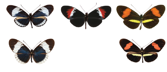
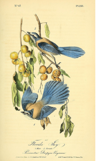
Positive assortative mating on the basis of a phenotype can create an excess of homozygotes. Heliconius butterflies are famous for their mimicry, where poisonous pairs of distantly related species mimic each others’ bright colour patterns and so share the benefits of being avoided by visual predators (Müllerian mimics). H. melpomene rosina and H. cydno chioneus are closely related species that co-occur in central Panama, but mimic different other co-occuring species (Figure \(\PageIndex{6}\) ). These differences in colouration pattern are due to a few loci with large phenotypic effects. The two species can hybridize and produce viable F1 hybrids. These F1 hybrids are heterozygotes at the colour loci, and their intermediate appearance means that they’re poor mimics and so are quickly eaten by predators. However, these heterzygote (F1) hybrids are very rare in nature Figure \(\PageIndex{7}\), as the parental species show strong positive assortatively mating based on colour pattern, based on genetic differences in mate preference .
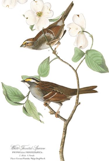
Disassortative mating, mating of unlike individuals, can lead to an excess of heterozygotes and a deficit of homozygotes. One example of very strong disassortative mating is offered by white-throated sparrows (Zonotrichia albicollis). In white-throated sparrows, there is a white-striped and a tan-striped morph, with female and male white-striped morphs have a much brighter white stripe and throat. There is very strong disassortative mating in this system, with 1099 out of 1116 nesting pairs consisting of one tan- and one white-striped morph and only 17 of these nesting pairs being different morphs . The difference between these morphs has a simple inheritance pattern, with white being due to a single dominant allele (called 2m) and tan color from a recessive allele called 2. Thus strong disassortative mating has a strong effect on the genotype frequencies:
| Tan | White | (Super)White |
|---|---|---|
| 2/2 | 2/2m | 2m/2m |
| 978 | 1011 | 3 |
There are almost no 2m homozygotes (so called Super white individuals) despite the 2m allele being common in the population (data from Tuttle et al., 2016, table S1).
Another important example of disassortative mating are mating type systems, which are present in many fungi, algae, and protozoa. Gametes of the same species can only fuse to form a zygote if they differ in mating type. The mating type of gametes is genetically controled by a mating type locus, and so individuals are nearly always heterozygous at this locus. In some groups of organisms, there are just two different alleles, in other clades these loci have tens or hundreds of alleles.
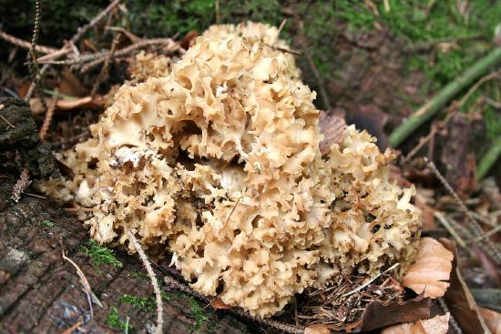
at up to 30lb and apparently taste like noodles. In a collection of 18 fruiting bodies from a Sparassis population, all individuals were heterozygotes for mating type and 17 different mating types were genetically identified (James, 2015; Martin and Gilbertson, 1978). (CC BY-SA 3.0; CC BY 3.0 via Wikipedia)
Allele sharing among related individuals and Identity by Descent
All of the individuals in a population are related to each other by a giant pedigree (family tree). For most pairs of individuals in a population these relationships are very distant (e.g. distant cousins), while some individuals will be more closely related (e.g. sibling/first cousins). All individuals are related to one another by varying levels of relatedness, or kinship. Related individuals can share alleles that have both descended from the shared common ancestor. To be shared, these alleles must be inherited through all meioses connecting the two individuals (e.g. surviving the \(\frac{1}{2}\) probability of segregation each meiosis). As closer relatives are separated by fewer meioses, closer relatives share more alleles. In Figure \(\PageIndex{10}\) we show the sharing of chromosomal regions between two cousins. As we’ll see, many population and quantitative genetic concepts rely on how closely related individuals are, and thus we need some way to quantify the degree of kinship among individuals.
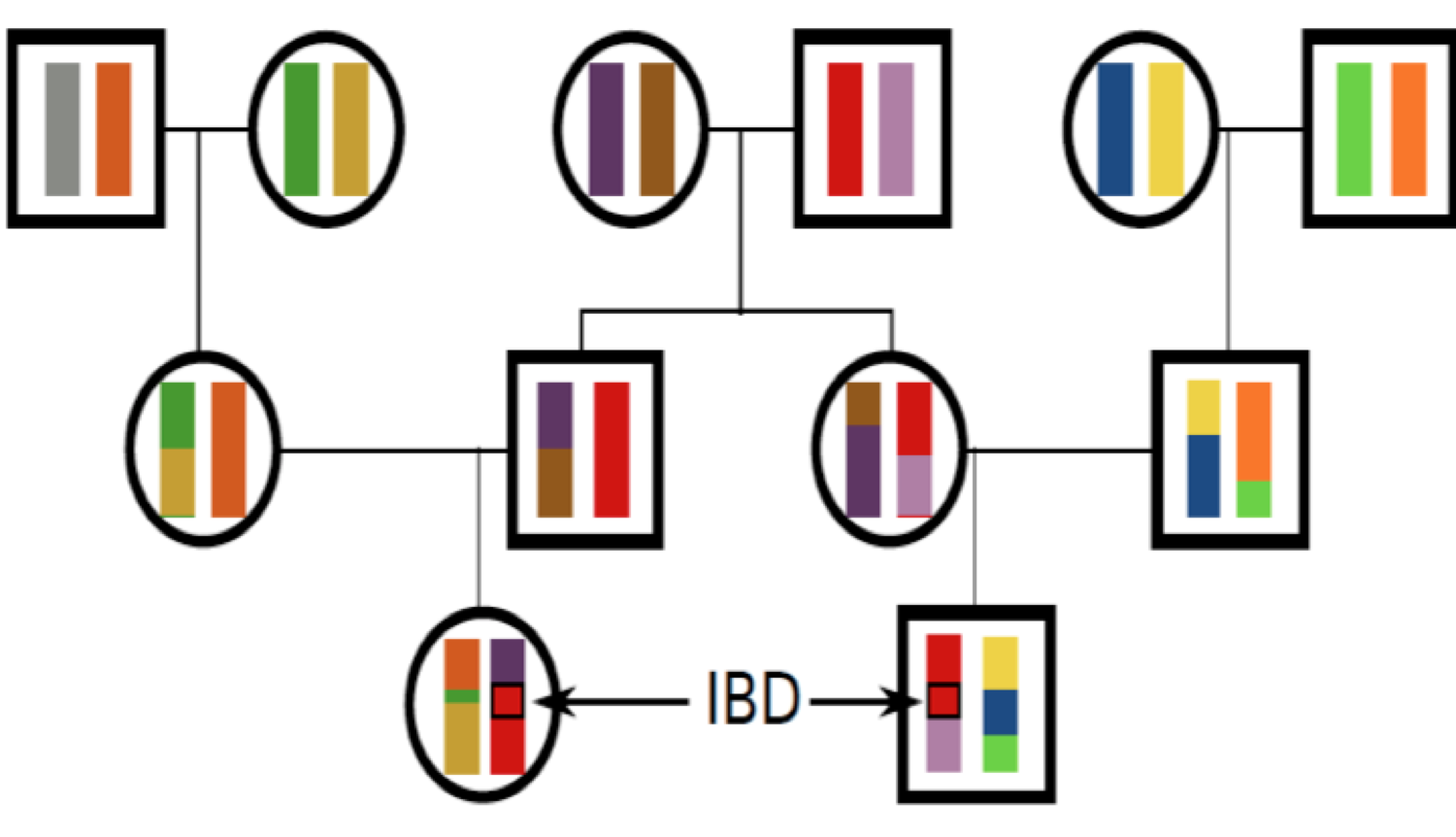
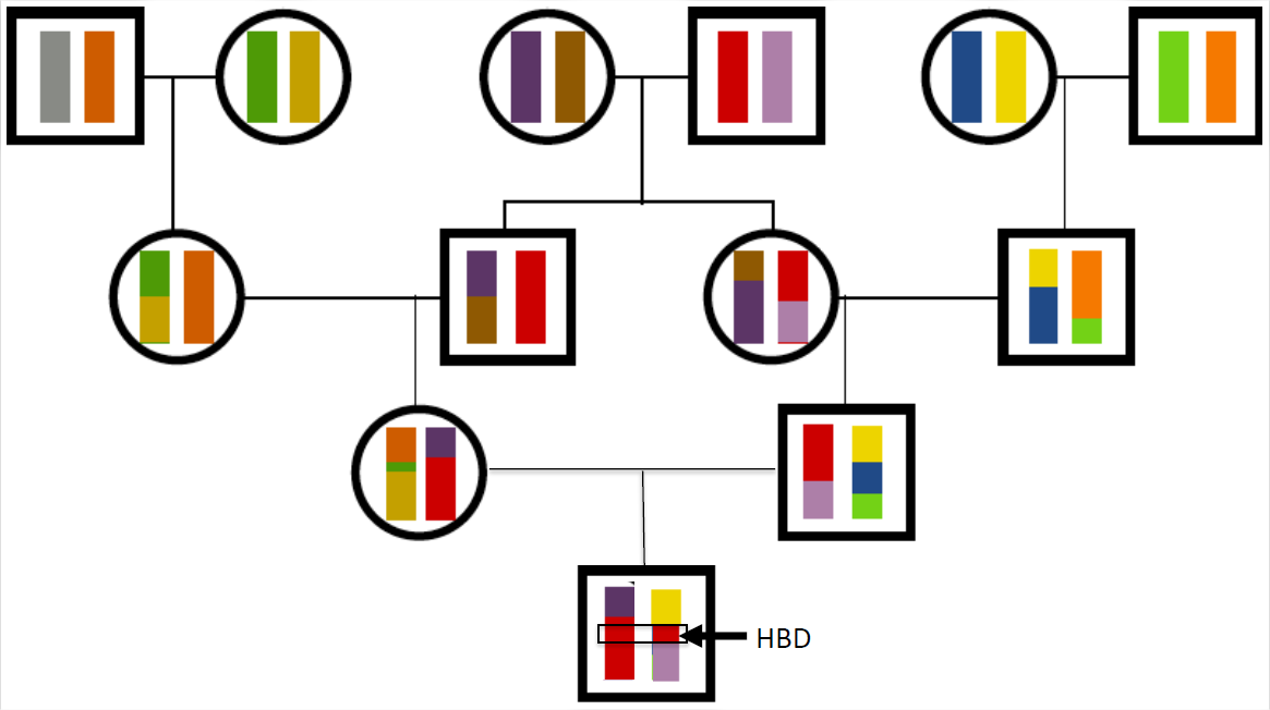
We will define two alleles to be identical by descent (IBD) if they are identical due to transmission from a common ancestor in the past few generations. For the moment, we ignore mutation, and we will be more precise about what we mean by ‘past few generations’ later on. For example, parent and child share exactly one allele identical by descent at a locus, assuming that the two parents of the child are randomly mated individuals from the population. In Figure \(\PageIndex{16}\), I show a pedigree demonstrating some configurations of IBD.
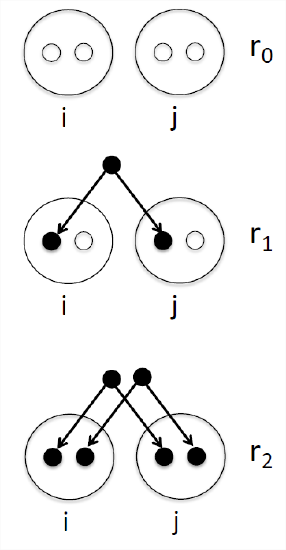
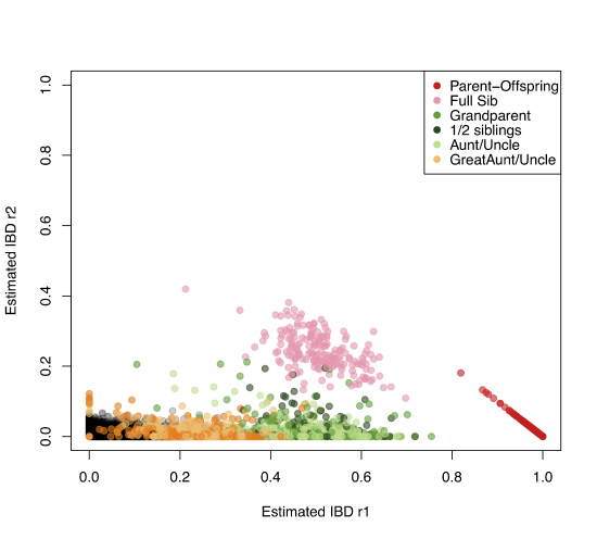
One summary of how related two individuals (let’s call them \(i\) and \(j\)) are is the probability that our pair of individuals share 0, 1, or 2 alleles identical by descent (see Figure \(\PageIndex{11}\)). We denote these identity-by-descent probabilities by \(r_0\), \(r_1\), and \(r_2\) respectively. See Table \(\PageIndex{4}\) for some examples. We can also interpret these probabilities as genome-wide averages. For example, on average, at a quarter of all their autosomal loci full-sibs share zero alleles identical by descent.
One summary of relatedness that will be important is the probability that two alleles (I & J) picked at random, one from each of the two different individuals \(i\) and \(j\), are identical by descent (\(P(\text{i & j IBD})\)). We call this quantity the coefficient of kinship of individuals \(i\) and \(j\), and denote it by \(F_{ij}\). It is calculated as
\[\begin{aligned} F_{ij} = & \mathbb{P}(\text{I & J IBD} )\\[4pt] =& \mathbb{P}(\text{I & J IBD} |~ \text{i & j 0 IBD}) \mathbb{P}(\text{i & j 0 IBD}) + \mathbb{P}(\text{I & J IBD} |~ \text{i & j 1 IBD}) \mathbb{P}(\text{i & j 1 IBD}) + \mathbb{P}(\text{I & J IBD} |~ \text{i & j 2 IBD}) \mathbb{P}(\text{i & j 2 IBD}) \label{eqn:coeffkinship_step}\\[4pt] = & 0 \times r_0 + \frac{1}{4} r_1 + \frac{1}{2} r_2. \label{eqn:coeffkinship}\end{aligned}\]
In the above step, \ref{eqn:coeffkinship_step}, we’re summing the conditional probability of alleles \(I\) & \(J\) being IBD over whether our individuals \(i\) & \(j\) share \(0\), \(1\), or \(2\) alleles IBD, an example of using the Law of Total Probability (see Appendix \ref{eqn:law_tot_prob}). We’ve then, in \ref{eqn:coeffkinship}, used the fact that we can calculate our condition probabilities of I & J being IBD using the rules of Mendelian transmision. Consider the probability \(P(\text{i & j IBD} |~ \text{i & j 1 IBD})\), i.e. that our pair of alleles (\(I\) & \(J\)) drawn from individuals \(i\) and \(j\) are IBD given that \(i\) and \(j\) share one allele IBD, this is a \(\frac{1}{4}\) as we need to draw the allele that is IBD from both \(i\) and \(j\), i.e. drawing both black alleles in the middle panel of Figure \ref{fig:IBD_0_1_2}, which happens with probability \(\frac{1}{2} \times \frac{1}{2}\). The coefficient of kinship will appear multiple times, in both our discussion of inbreeding and in the context of phenotypic resemblance between relatives.
Table \(\PageIndex{4}\): Probability that two individuals (i and j) of a given re- lationship share 0, 1, or 2 alleles identical by descent on the autosomes. ∗Assuming that our individuals are outbred and that this the only close relationship the pair shares.
| Relationship (i,j)\(^{*}\) | \(\mathbb{P}(\text{i & j 0 IBD})\) | \(\mathbb{P}(\text{i & j 1 IBD})\) | \(P(\text{i & j 2 IBD})\) | \(\mathbb{P}(\text{i & j IBD} )\) |
|---|---|---|---|---|
| Relationship (i,j)\(^{*}\) | \(r_0\) | \(r_1\) | \(r_2\) | \(F_{ij}\) |
| parent–child | 0 | 1 | 0 | |
| full siblings | ||||
| Monozygotic twins | 0 | 0 | 1 | |
| \(1^{st}\) cousins | 0 |
What are \(r_0\), \(r_1\), and \(r_2\) for \(\frac{1}{2}\) sibs? (\(\frac{1}{2}\) sibs share one parent but not the other).
Explain in words why \(\mathbb{P}(\text{i & j IBD} |~ \text{i & j 2 IBD}) = \frac{1}{2}\).
Genotypic sharing between pairs of individuals
Our \(r\) coefficients are going to have various uses. For example, they allow us to calculate the probability of the genotypes of a pair of relatives. Consider a biallelic locus where allele \(A_1\) is at frequency \(p\), and two individuals who have IBD allele sharing probabilities \(r_0\), \(r_1\), \(r_2\). What is the overall probability that these two individuals are both homozygous for allele 1? Well that’s
\[\begin{aligned} \mathbb{P}(\textrm{both } A_1 A_1) = & \mathbb{P}(\textrm{both } A_1 A_1 | 0 \text{ alleles } \mathrm{IBD}) \mathbb{P}(0 \text{ alleles } \mathrm{IBD}) + \mathbb{P}(\textrm{both } A_1 A_1 | 1 \text{ allele }IBD) \mathbb{P}(1\text{ allele }IBD) + \mathbb{P}(\textrm{both } A_1 A_1 | 2 \text{ alleles }IBD) \mathbb{P}(2\text{ alleles }IBD)\end{aligned}\]
Or, in our \(r_0\), \(r_1\), \(r_2\) notation:
\[\begin{aligned} \mathbb{P}(\textrm{both } A_1 A_1) = & \mathbb{P}(\textrm{both } A_1 A_1 | \textrm{0 alleles IBD}) r_0 + \mathbb{P}(\textrm{both } A_1 A_1 | \textrm{1 alleles IBD}) r_1 + \mathbb{P}(\textrm{both } A_1 A_1 | \textrm{2 alleles IBD}) r_2 \label{eqn:initial_relly_IBD_calc}\end{aligned}\]
If our pair of relatives share \(0\) alleles IBD, then the probability that they are both homozygous is \(\mathbb{P}(\textrm{both } A_1 A_1 | \text{0 alleles IBD}) =p^2 \times p^2\), as all four alleles represent independent draws from the population. If they share \(1\) allele IBD, then the shared allele is of type \(A_1\) with probability \(p\), and then the other non-IBD allele, in both relatives, also needs to be \(A_1\) which happens with probability \(p^2\), so \(\mathbb{P}(\textrm{both } A_1 A_1 | \text{1 alleles IBD})=p \times p^2\). Finally, our pair of relatives can share two alleles IBD, in which case \(\mathbb{P}(\textrm{both } A_1 A_1 | \text{2 alleles IBD}) = p^2\), because if one of our individuals is homozygous for the \(A_1\) allele, both individuals will be. Putting this all together our \ref{eqn:initial_relly_IBD_calc} becomes
\[\mathbb{P}(\textrm{both } A_1 A_1) = p^4 r_0 + p^3 r_1 + p^2 r_2 \label{eqn:IBD_relly_calc}\]
Note that for specific cases we could also calculate this by summing over all the possible genotypes their shared ancestor(s) had; however, that would be much more involved and not as general as the form we have derived here.
We can write out terms like \ref{eqn:IBD_relly_calc} for all of the possible configurations of genotype sharing/non-sharing between a pair of individuals. Based on this we can write down the expected number of polymorphic sites where our individuals are observed to share 0, 1, or 2 alleles.
The genotype of our suspect in Question \ref{Q:CODIS} turns out to be 100/80 for D16S539 and 70/80 at TH01. The suspect is not a match to the DNA from the crime scene; however, they could be a sibling.Calculate the joint probability of observing the genotype from the crime and our suspect:
- Assuming that they share no close relationship.
- Assuming that they are full sibs.
- Briefly explain your findings.
There’s a variety of ways to estimate the relationships among individuals using genetic data. An example of using allele sharing to identify relatives is offered by the work of Nancy Chen . has collected genotyping data from thousands of Florida Scrub Jays at over ten thousand loci. These Jays live at the Archbold field site, and have been carefully monitored for many decades allowing the pedigree of many of the birds to be known. Using these data, she estimates allele frequencies at each locus. Then by equating the observed number of times that a pair of individuals share \(0\), \(1\), or \(2\) alleles to the theoretical expectation, she estimates the probability of \(r_0\), \(r_1\), and \(r_2\) for each pair of birds. A plot of these are shown in Figure \(\PageIndex{13}\), showing how well the estimates match those known from the pedigree.
Sharing of genomic blocks among relatives
We can more directly see the sharing of the genome among close relatives using high-density SNP genotyping arrays. In Figure \ref{fig:first_cousin_IBD} we show a simulation of first cousins’ genomic sharing from their shared grandmother. Colored purple are regions where they have matching genomic material, due to having inherited it IBD from their shared grandmother.
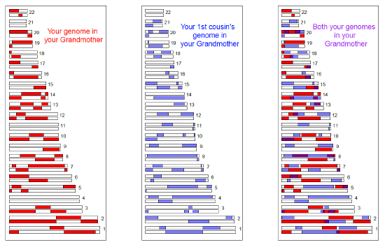
First cousins will share at least one allele of your genotype at all of the polymorphic loci in these purple regions. There’s a range of methods to detect such sharing. One way is to look for unusually long stretches of the genome where two individuals are never homozygous for different alleles. By identifying pairs of individuals who share an unusually large number of such putative IBD blocks, we can hope to identify unknown relatives in genotyping datasets. In fact, companies like 23&me and Ancestry.com use signals of IBD to help identify family ties.
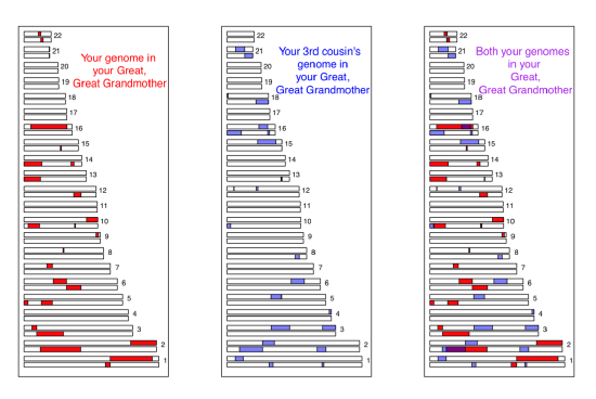
As another example, consider the case of third cousins. You share one of eight sets of great-great-grandparents with each of your (likely many) third cousins. On average, you and each of your third cousins each inherit one-sixteenth of your genome from each of those two great-great-grandparents. This turns out to imply that on average, a little less than one percent of your and your third cousin’s genomes (\(2 \times (1/16)^2 =0.78\%\)) will be identical by virtue of descent from those shared ancestors. A simulated example where third cousins share blocks of their genome (on chromosome 16 and 2) due to their great-great-grandmother is shown in Figure \(\PageIndex{14}\).
Note how if you compare Figure \(\PageIndex{15}\) and Figure \(\PageIndex{14}\), individuals inherit less IBD from a shared great-great-grandmother than from a shared grandmother, as they inherit from more total ancestors further back. Also notice how the sharing occurs in shorter genomic blocks, as it has passed through more generations of recombination during meiosis. These blocks are still detectable, and so third cousins can be detected using high-density genotyping chips, allowing more distant relatives to be identified than single marker methods alone. More distant relations than third cousins, e.g. fourth cousins, start to have a significant probability of sharing none of their genome IBD. But you have many fourth cousins, so you will share some of your genome IBD with some of them; however, it gets increasingly hard to identify the degree of relatedness from genetic data the deeper in the family tree this sharing goes.
Inbreeding
We can define an inbred individual as an individual whose parents are more closely related to each other than two random individuals drawn from some reference population.
When two related individuals produce an offspring, that individual can receive two alleles that are identical by descent, i.e. they can be homozygous by by descent (sometimes termed autozygous), due to the fact that they have two copies of an allele through different paths through the pedigree. This increased likelihood of being homozygous relative to an outbred individual is the most obvious effect of inbreeding. It is also the one that will be of most interest to us, as it underlies a lot of our ideas about inbreeding depression and population structure. For example, in Figure \(\PageIndex{16}\) our offspring of first cousins is homozygous by descent having received the same IBD allele via two different routes around an inbreeding loop.
As the offspring receives a random allele from each parent (\(i\) and \(j\)), the probability that those two alleles are identical by descent is equal to the kinship coefficient \(F_{ij}\) of the two parents (\ref{eqn:coeffkinship}). This follows from the fact that the genotype of the offspring is made by sampling an allele at random from each of our parents.
| \(f_{11}\) | \(f_{12}\) | \(f_{22}\) |
|---|---|---|
| \((1-F) p^2 + F p\) | \((1-F) 2pq\) | \((1-F) q^2 + F q\) |
The only way the offspring can be heterozygous (\(A_1 A_2\)) is if their two alleles at a locus are not IBD (otherwise they would necessarily be homozygous). Therefore, the probability that they are heterozygous is
\[\mathbb{P}(A_1 A_2) = \mathbb{P}(A_1 A_2 |\textrm{I & J not IBD} ) \P (\textrm{I & J not IBD} ) = 2p q (1-F_{ij}) , \label{eq:hetGenHW}\]
The offspring can be homozygous for the \(A_1\) allele in two different ways. They can have two non-IBD alleles that are not IBD but happen to be of the allelic type \(A_1\), or their two alleles can be IBD, such that they inherited allele \(A_1\) by two different routes from the same ancestor. Thus, the probability that an offspring is homozygous for \(A_1\) is
\[\begin{aligned} P(A_1 A_1) & = \mathbb{P}(A_1 A_1 |\textrm{I & J not IBD} ) \P (\textrm{i & j not IBD} ) + \mathbb{P}(A_1 A_1 |\textrm{i & j IBD} ) \P (\textrm{i & j IBD}) \nonumber\\ &= p^2(1-F_{ij}) + pF_{ij}.\end{aligned}\]
using the Law of Total Probability (see Appendix \ref{eqn:law_tot_prob}). Therefore, the frequencies of the three possible genotypes can be written as given in Table \(\PageIndex{5}\), which provides a generalization of the Hardy–Weinberg proportions.
The frequency of the \(A_1\) allele is \(p\) at a biallelic locus. Assume that our population is randomly mating and that the genotype frequencies in the population follow from HW. We select two individuals at random to mate from this population. We then mate the children from this cross. What is the probability that the child from this full sib-mating is homozygous?
Multiple inbreeding loops in a pedigree
Up to this point we have assumed that there is at most one inbreeding loop in the recent family history of our individuals, i.e. the parents of our inbred individual have at most one recent genealogical connection. However, an individual who has multiple inbreeding loops in their pedigree can be homozygous by descent thanks to receiving IBD alleles via multiple different different loops. To calculate inbreeding in pedigrees of arbitrary complexity, we can extend beyond our original relatedness coefficients \(r_0\), \(r_1\), and \(r_2\) to account for higher order sharing of alleles IBD among relatives. For example, we can ask, what is the probability that both of the alleles in the first individual are shared IBD with one allele in the second individual? There are nine possible relatedness coefficients in total to completely describe kinship between two diploid individuals, and we won’t go in to them here as it’s a lot to keep track of. However, we will show how we can calculate the inbreeding coefficient of an individual with multiple inbreeding loops more directly.
Let’s say the parents of our inbred individual (B and C) have \(K\) shared ancestors, i.e. individuals who appear in both B and C’s recent family trees. We denote these shared ancestors by \(A_1, \dots,A_K\), and we denote by \(n\) the total number of individuals in the chain from B to C via ancestor \(A_i\), including B, C, and \(A_i\). For example, if B is C’s aunt, then B and C share two ancestors, which are B’s parents and, equivalently, C’s grandparents. In this case, there are n=4 individuals from B to C through each of these two shared ancestor. In the general case, the kinship coefficient of B and C, i.e. the inbreeding coefficient of their child, is
\[F = \sum_{i=1}^K \frac{1}{2^{n_i}} \big( 1+ f_{A_i} \big) \label{eqn:inbreeding_over_ancs}\]
where \(f_{A_i}\) is the inbreeding coefficient of the ancestor \(A_i\). What’s happening here is that we sum over all the mutually-exclusive paths in the pedigree through which B and C can share an allele IBD. With probability \(\frac{1}{2^{n_i}}\), a pair of alleles picked at random from B and C is descended from the same ancestral allele in individual \(A_i\), in which case the alleles are IBD. However, even if B inherits the maternal allele and C inherits the paternal allele of shared ancestor \(A_i\), if \(A_i\) was themselves inbred, with probability \(f_{A_i}\) those two alleles are themselves IBD. Thus a shared inbred ancestor further increases the kinship of B and C.
Multiple inbreeding loops increase the probability that a child is homozygous by descent at a locus, which can be calculated simply by plugging in \(F\), the child’s inbreeding coefficient, into our generalized HW equation.
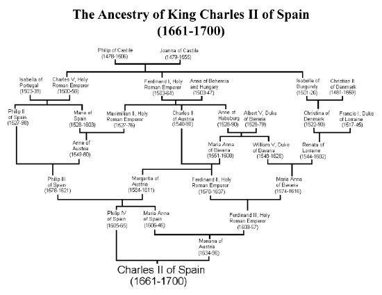
As one extreme example of the impact of multiple inbreeding loops in an individual’s pedigree, let’s consider king Charles II of Spain, the last of the Spanish Habsburgs. Charles was the son of Philip IV of Spain and Mariana of Austria, who were uncle and niece. If this were the only inbreeding loop, then Charles would have had an inbreeding coefficient of \(\frac{1}{8}\). Unfortunately for Charles, the Spanish Habsburgs had long kept wealth and power within their family by arranging marriages between close kin. The pedigree of Charles II is shown in Figure \(\PageIndex{17}\), and multiple inbreeding loops are apparent. For example, Phillip III, Charles II’s grandfather and great-grandfather, was himself a child of an uncle-niece marriage.
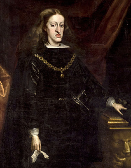
calculated that Charles II had an inbreeding coefficient of \(0.254\), equivalent to a full-sib mating, thanks to all of the inbreeding loops in his pedigree. Therefore, he is expected to have been homozygous by descent for a full quarter of his genome. As we’ll talk about later in these notes, this means that Charles may have been homozygous for a number of recessive disease alleles, and indeed he was a very sickly man who left no descendants due to his infertility. Thus plausibly the end of one of the great European dynasties came about through inbreeding.
Calculating inbreeding coefficients from genetic data
If the observed heterozygosity in a population is \(H_O\), and we assume that the generalized Hardy–Weinberg proportions hold, we can set \(H_O\) equal to \(f_{12}\), and solve Equation \ref{eq:hetGenHW} for \(F\) to obtain an estimate of the inbreeding coefficient as
\[\hat{F} = 1-\frac{f_{12}}{2pq} = \frac{2pq - f_{12}}{2pq}. \label{eqn:Fhat}\]
As before, \(p\) is the frequency of allele \(A_{1}\) in the population. This can be rewritten in terms of the observed heterozygosity (\(H_O\)) and the heterozygosity expected in the absence of inbreeding, \(H_E=2pq\), as
\[\hat{F} = \frac{H_E-H_O}{H_E} = 1 - \frac{H_O}{H_E}. \label{eqn:FhatHO}\]
Hence, \(\hat{F}\) quantifies the deviation due to inbreeding of the observed heterozygosity from the one expected under random mating, relative to the latter.
Suppose the following genotype frequencies were observed for an esterase locus in a population of Drosophila (A denotes the “fast" allele and B denotes the “slow" allele):
| AA | AB | BB |
|---|---|---|
| 0.6 | 0.2 | 0.2 |
What is the estimate of the inbreeding coefficient at the esterase locus?
If we have multiple loci, we can replace \(H_O\) and \(H_E\) by their means over loci, \(\bar{H}_O\) and \(\bar{H}_E\), respectively. Note that, in principle, we could also calculate \(F\) for each individual locus first, and then take the average across loci. However, this procedure is more prone to introducing a bias if sample sizes vary across loci, which is not unlikely when we are dealing with real data.
Genetic markers are commonly used to estimate inbreeding for wild and/or captive populations of conservation concern. As an example of this, consider the case of the Mexican wolf (Canis lupus baileyi), a sub-species of gray wolf.
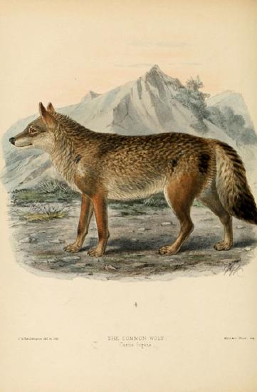
They were extirpated in the wild during the mid-1900s due to hunting, and the remaining five Mexican wolves in the wild were captured to start a breeding program. estimated the current-day, average expected heterozygosity to be \(0.18\), based on allele frequencies at over forty thousand SNPs. However, the average Mexican wolf individual was only observed to be heterozygous at \(12\%\) of these SNPs. Therefore, the average inbreeding coefficient for the Mexican wolf is \(\hat{F} = 1 -\frac{0.12}{0.18}\), i.e. \(\sim 33 \%\) of a lobo’s genome is homozygous due to recent inbreeding in their pedigree.
Genomic blocks of homozygosity due to inbreeding.
As we saw above, close relatives are expected to share alleles IBD in large genomic blocks. Thus, when related individuals mate and transmit alleles to an inbred offspring, they transmit these alleles in big blocks through meiosis. As an example, let’s return to the case of our hypothetical first cousins from Figure \ref{fig:IBD_cousins_chr_cartoon}. If this pair of individuals had a child, one possible pattern of genetic transmission is shown in Figure \(\PageIndex{20}\). The child has inherited the red stretch of chromosome via two different routes through their predigree from the grandparents. This is an example of an autozygous segment, where the child is homozygous by descent at all of the loci in this red region.
The inbreeding coefficient of the child sets the proportion of their genome that will be in these autozygous segments. For example, a child of first full cousins is expected to have \(1/16\) of their genome in these segments. The more distant the loop in the pedigree, the more meioses that chromosomes have been through and the shorter individual blocks will be. A child of first cousins will have longer blocks than a child of second cousins, for example.
Individuals with multiple inbreeding loops in their family tree can have a high inbreeding coefficient due to the combined effect of many small blocks of autozygosity. For example, Charles II had an inbreeding coefficient that is equivalent to that of the child of full-sibs, with a quarter of his genome expected to homozygous by descent, but this would be made up of many shorter blocks.
We can hope to detect these blocks by looking for unusually long genomic runs of homozygosity (ROH) sites in an individual’s genome. One way to estimate an individual’s inbreeding coefficient is then to total up the proportion of an individual’s genome that falls in such ROH regions. This estimate is called \(F_{ROH}\).
An example of using \(F_{ROH}\) to study inbreeding comes from the work of Sams and Boyko (2018b), who identified runs of homozygosity in 2,500 dogs, ranging from 500kb up to many megabases. Figure \(\PageIndex{21}\) shows the distribution of FROH of individuals in each dog breed for the X and autosome. In Figure \(\PageIndex{23}\) this is broken down by the length of ROH segments.
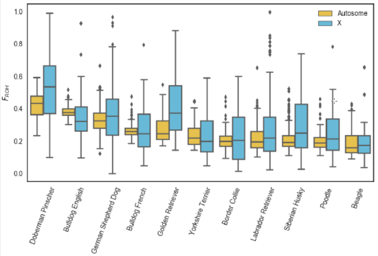
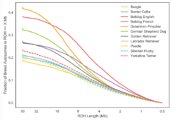
Dog breeds have been subject to intense breeding that has resulted in high levels of inbreeding. Of the population samples examined, Doberman Pinschers have the highest levels of their genome in runs of homozygosity (\(F_{ROH}\)), somewhat higher than English bulldogs. In Figure \(\PageIndex{23}\) we can see that English bulldogs have more short ROH than Doberman Pinschers, but that Doberman Pinschers have more of their genome in very large ROH (\(>16 Mb\)). This suggests that English bulldogs have had long history of inbreeding as they have many small blocks, but that Doberman Pinschers have a lot of recent inbreeding as their autozygosity is contained in long blocks relatively unbroken by recombination.
Summary
- This chapter developed the relationship between allele frequencies and genotype frequencies within a generation and among relatives.
- Under random mating, we derived expectations of the genotype frequencies (Hardy-Weinberg), and we can identify deviations away from these expectations.
- Identity by descent (IBD) refers to the sharing of alleles due to a recent shared biological relationship.
- We can predict the probability and expected level of sharing of alleles IBD among pairs of relatives using mendelian transmission probabilities (as contained in coefficients \(r_0\), \(r_1\), and \(r_2\)). One useful summary of relatedness for a pair of individuals is the kinship coefficient \(F_{i,j}\).
- We can also learn about genetic relationships from the sharing of genomic segments among relatives, with many long shared segments revealing a closer relationship.
- An inbred individual has parents who are more closely related than random draws from some reference population.
- Inbreeding results in decreased heterozygosity and a complementary increase in homozygosity. We can use the kinship coefficient of the parents to estimate the distortion away from Hardy-Weinberg and the expected level of heterozygosity.
- Inbreeding coefficients can be calculated from genetic data, either for multiple individuals at a single locus or for multiple loci for a single individual.
Calculate \(r_{0}\), \(r_{1}\), \(r_{2}\) and the coefficient of kinship \(F\) between:
- A grandparent and their grandchild
- A great grandparent and their great grandchild
- Full siblings
- A great aunt and her grand nephew (your great aunt = your parent’s aunt)
You are studying a codominant flower colour polymorphism. Skipping through a meadow of flowers you and compile the following data:
| red | pink | white |
| 200 | 100 | 200 |
- What frequencies would you expect at this locus under Hardy-Weinberg equilibrium?
- Calculate the inbreeding coefficient at this locus.
- Name two distinct processes that could lead to the deviation you see, and describe how they would result in a deficit of heterozygotes.
What are the relatedness coefficients of the X chromosome between:
- Two male full siblings?
- Two female full siblings?
- What is the probability that a female offspring of a full sib mating is homozygous by descent at a locus on her X chromosome?
You are studying the wing spot polymorphism in a butterfly species. From crosses in the lab you find that the presence of wing spots is determined by a dominant allele.
You collect 100 butterflies, 84 of them have the wing spots. What is the frequency of the wing-spot allele? What assumption did you have to make to come to your answer?
An allele has frequency of \(0.001\) in the population. What is the probability that both you and your first (full) cousin are heterozygote for the allele?
The kinship coefficient of the parents is the inbreeding coefficient of the offspring. Explain, with reference to the weighting of relatedness coefficients in the inbreeding coefficient, why the inbreeding coefficient is the probability that a locus is homozygous by descent.
In terms of identity by descent, explain why multiple inbreeding loops in an individual’s pedigree lead to higher levels of inbreeding.