1.7: Probabilities in genetics

Introduction

The Punnett square is a valuable tool, but it's not ideal for every genetics problem. For instance, suppose you were asked to calculate the frequency of the recessive class not for an Aa x Aa cross, not for an AaBb x AaBb cross, but for an AaBbCcDdEe x AaBbCcDdEe cross. If you wanted to solve that question using a Punnett square, you could do it – but you'd need to complete a Punnett square with 1024 boxes. Probably not what you want to draw during an exam, or any other time, if you can help it!

The five-gene problem above becomes less intimidating once you realize that a Punnett square is just a visual way of representing probability calculations. Although it’s a great tool when you’re working with one or two genes, it can become slow and cumbersome as the number goes up. At some point, it becomes quicker (and less error-prone) to simply do the probability calculations by themselves, without the visual representation of a clunky Punnett square. In all cases, the calculations and the square provide the same information, but by having both tools in your belt, you can be prepared to handle a wider range of problems in a more efficient way.

In this article, we’ll review some probability basics, including how to calculate the probability of two independent events both occurring (event X and event Y) or the probability of either of two mutually exclusive events occurring (event X or event Y). We’ll then see how these calculations can be applied to genetics problems, and, in particular, how they can help you solve problems involving relatively large numbers of genes.

[Solution to the five-gene cross problem]

In this problem, we’re supposed to find the frequency of the recessive class among the offspring of an AaBbCcDdEe x AaBbCcDdEe cross – that is, the frequency of aabbccddee individuals. How do we get an aabbccddee individual? There’s only one way for that to happen: both parents must contribute an abcde gamete.

What, then, is the probability that one of the parents will make an abcde gamete? Both parents are heterozygous for all five genes, so there’s a 1/2 chance of getting the recessive (lowercase) allele for any one gene. To get our desired gamete, we need all five genes in recessive form (a and b and c and d and e). This is a case where we can apply the product rule, which states that the probability of event X and event Y happening is the product of their individual probabilities (probability of X times probability of Y), assuming that X and Y are independent events. Thus, the overall probability of one parent producing an abcde gamete is:

Probability of abcde gamete = (probability of a) x (probability of b) x (probability of c) x (probability of d) x (probability of e)

\(P(abcde)=P(a)\cdot P(b)\cdot P(c)\cdot P(d)\cdot P(e)\)

\(P(abcde)=(1/2)\cdot (1/2)\cdot (1/2)\cdot (1/2)\cdot (1/2)=(1/2)^5=1/32\)

If that’s the probability of one parent making an abcde gamete, what’s the likelihood of both parents doing so? Again, we can apply the "and" rule (product rule), since we need both parent 1 and parent 2 to make an abcde gamete in order to get our target recessive homozygote. Thus, the overall probability is:

Probability of aabbccddee individual = (probability of parent 1 making an abcde gamete) x (probability of parent 2 making an abcde gamete)

\(P(aabbccddee)=P(abcde_\text{parent A})\cdot P(abcde_\text{parent B})\)

\(P(aabbccddee)=(1/32)\cdot (1/32)=1/1024\)

That’s our overall probability for a recessive homozygote for all five genes.

The 1/1024 probability corresponds to 1 box out of the 1024 boxes of the Punnett square you’d have to draw to represent this cross. The probability calculation is the same calculation we’d implicitly do by drawing the Punnett square, just faster and with fewer chances for mistakes.

Probability basics

Probabilities are mathematical measures of likelihood. In other words, they’re a way of quantifying (giving a specific, numerical value to) how likely something is to happen. A probability of 1 for an event means that it is guaranteed to happen, while a probability of 0 for an event means that it is guaranteed not to happen. A simple example of probability is having a 1/2 chance of getting heads when you flip a coin, as Sal explains in this intro to probability video.

Probabilities can be either empirical, meaning that they are calculated from real-life observations, or theoretical, meaning that they are predicted using a set of rules or assumptions.

• The empirical probability of an event is calculated by counting the number of times that event occurs and dividing it by the total number of times that event could have occurred. For instance, if the event you were looking for was a wrinkled pea seed, and you saw it 1,850 times out of the 7,324 total seeds you examined, the empirical probability of getting a wrinkled seed would be 1,850/7,324 = 0.253, or very close to 1 in 4 seeds.
• The theoretical probability of an event is calculated based on information about the rules and circumstances that produce the event. It reflects the number of times an event is expected to occur relative to the number of times it could possibly occur. For instance, if you had a pea plant heterozygous for a seed shape gene (Rr) and let it self-fertilize, you could use the rules of probability and your knowledge of genetics to predict that 1 out of every 4 offspring would get two recessive alleles (rr) and appear wrinkled, corresponding to a 0.25 (1/4) probability. We’ll talk more below about how to apply the rules of probability in this case.

In general, the larger the number of data points that are used to calculate an empirical probability, such as shapes of individual pea seeds, the more closely it will approach the theoretical probability.

The product rule

One probability rule that's very useful in genetics is the product rule, which states that the probability of two (or more) independent events occurring together can be calculated by multiplying the individual probabilities of the events. For example, if you roll a six-sided die once, you have a 1/6 chance of getting a six. If you roll two dice at once, your chance of getting two sixes is: (probability of a six on die 1) x (probability of a six on die 2) = (1/6) ⋅ (1/6) = 1/36.

In general, you can think of the product rule as the “and” rule: if both event X and event Y must happen in order for a certain outcome to occur, and if X and Y are independent of each other (don’t affect each other’s likelihood), then you can use the product rule to calculate the probability of the outcome by multiplying the probabilities of X and Y.

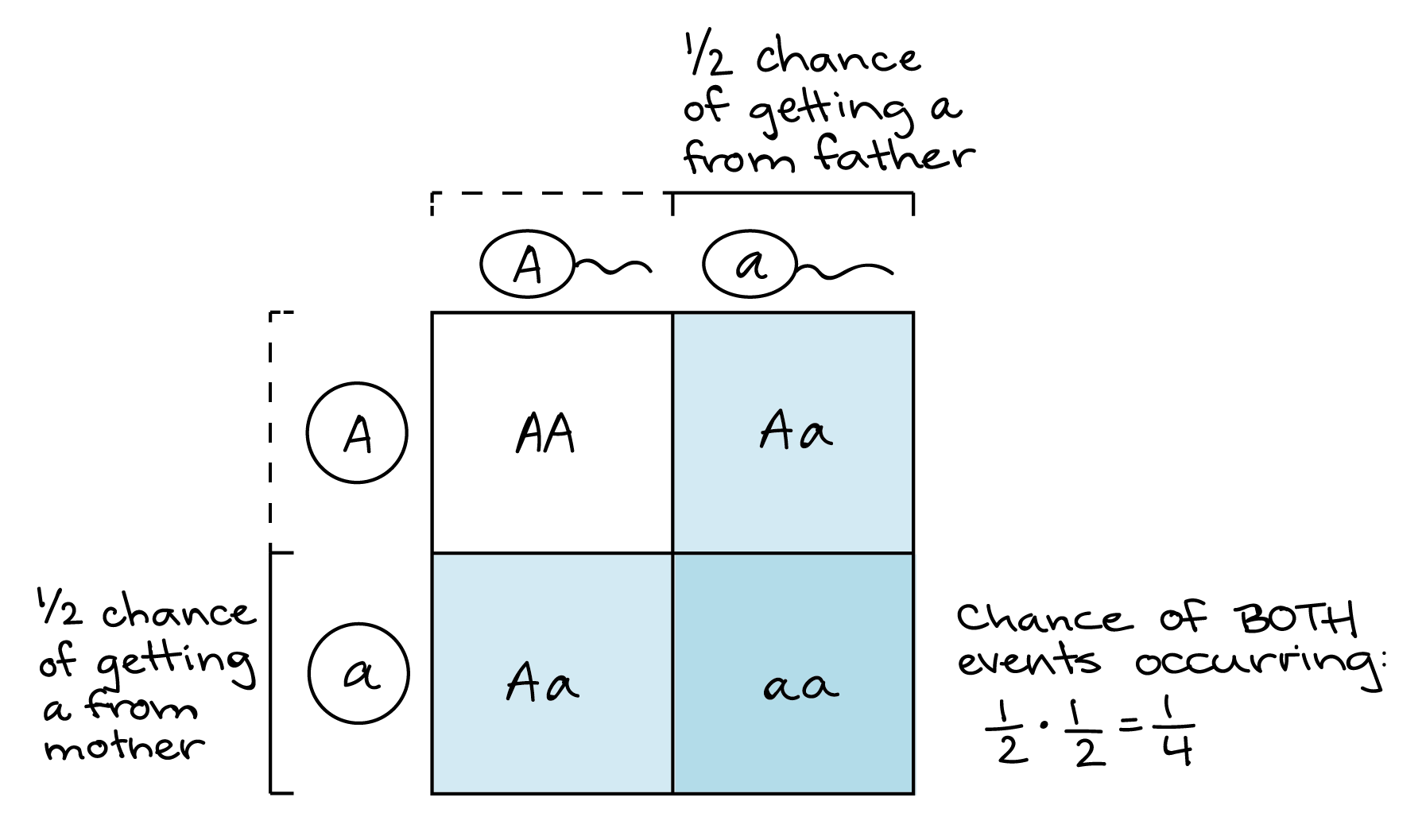
We can use the product rule to predict frequencies of fertilization events. For instance, consider a cross between two heterozygous (Aa) individuals. What are the odds of getting an aa individual in the next generation? The only way to get an aa individual is if the mother contributes an a gamete and the father contributes an a gamete. Each parent has a 1/2 chance of making an a gamete. Thus, the chance of an aa offspring is: (probability of mother contributing a) x (probability of father contributing a) = (1/2) ⋅ (1/2) = 1/4.

This is the same result you’d get with a Punnett square, and actually the same logical process as well—something that took me years to realize! The only difference is that, in the Punnett square, we'd do the calculation visually: we'd represent the 1/2 probability of an a gamete from each parent as one out of two columns (for the father) and one out of two rows (for the mother). The 1-square intersect of the column and row (out of the 4 total squares of the table) represents the 1/4 chance of getting an a from both parents.

The sum rule of probability

In some genetics problems, you may need to calculate the probability that any one of several events will occur. In this case, you’ll need to apply another rule of probability, the sum rule. According to the sum rule, the probability that any of several mutually exclusive events will occur is equal to the sum of the events’ individual probabilities.

For example, if you roll a six-sided die, you have a 1/6 chance of getting any given number, but you can only get one number per roll. You could never get both a one and a six at the same time; these outcomes are mutually exclusive. Thus, the chances of getting either a one or a six are: (probability of getting a 1) + (probability of getting a 6) = (1/6) + (1/6) = 1/3.

You can think of the sum rule as the “or” rule: if an outcome requires that either event X or event Y occur, and if X and Y are mutually exclusive (if only one or the other can occur in a given case), then the probability of the outcome can be calculated by adding the probabilities of X and Y.

As an example, let's use the sum rule to predict the fraction of offspring from an Aa x Aa cross that will have the dominant phenotype (AA or Aa genotype). In this cross, there are three events that can lead to a dominant phenotype:

• Two A gametes meet (giving AA genotype), or
• A gamete from Mom meets a gamete from Dad (giving Aa genotype), or
• a gamete from Mom meets A gamete from Dad (giving Aa genotype)

In any one fertilization event, only one of these three possibilities can occur (they are mutually exclusive).

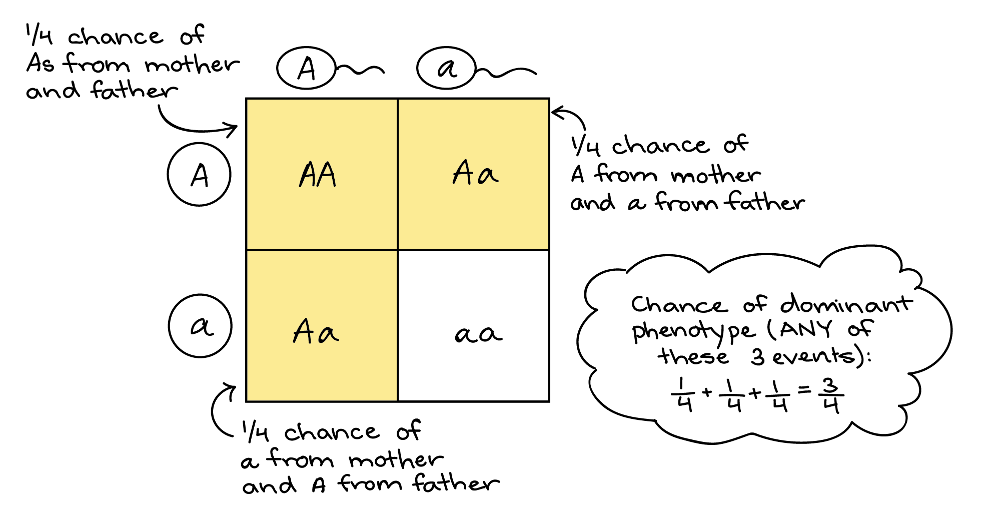
Since this is an “or” situation where the events are mutually exclusive, we can apply the sum rule. Using the product rule as we did above, we can find that each individual event has a probability of 1/4. So, the probability of offspring with a dominant phenotype is: (probability of A from Mom and A from Dad) + (probability of A from Mom and a from Dad) + (probability of a from Mom and A from Dad) = (1/4) + (1/4) + (1/4) = 3/4.

Once again, this is the same result we’d get with a Punnett square. One out of the four boxes of the Punnett square holds the dominant homozygote, AA. Two more boxes represent heterozygotes, one with a maternal A and a paternal a, the other with the opposite combination. Each box is 1 out of the 4 boxes in the whole Punnett square, and since the boxes don't overlap (they’re mutually exclusive), we can add them up (1/4 + 1/4 + 1/4 = 3/4) to get the probability of offspring with the dominant phenotype.

The product rule and the sum rule

Product rule	Sum rule
For independent events X and Y, the probability (\(P\)) of them both occurring (X and Y) is \(P(X)\cdot P(Y)\).	For mutually exclusive events X and Y, the probability (\(P\)) that one will occur (X or Y) is \(P(X)+P(Y)\).

Applying probability rules to dihybrid crosses

Direct calculation of probabilities doesn’t have much advantage over Punnett squares for single-gene inheritance scenarios. (In fact, if you prefer to learn visually, you may find direct calculation trickier rather than easier.) Where probabilities shine, though, is when you’re looking at the behavior of two, or even more, genes.

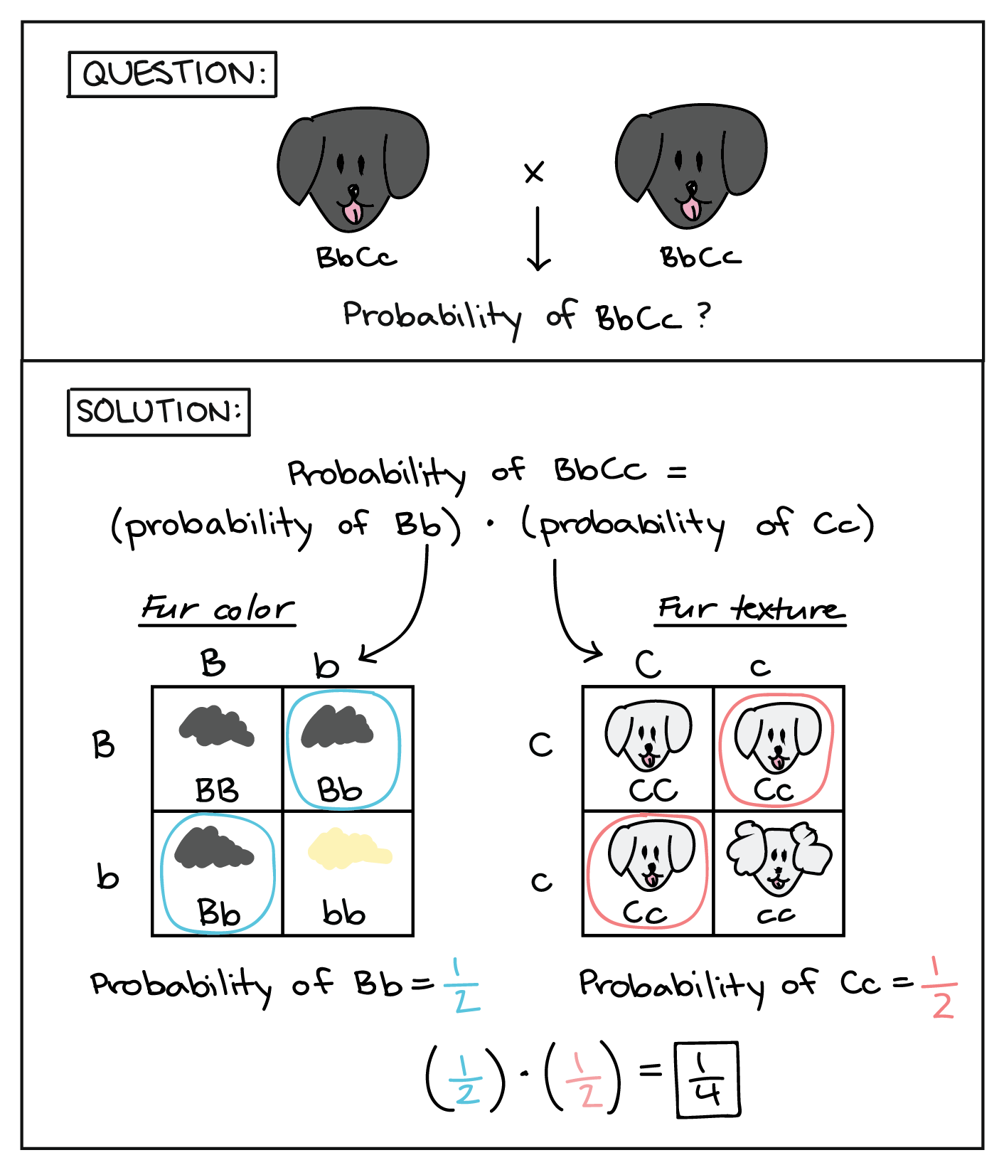
For instance, let’s imagine that we breed two dogs with the genotype BbCc, where dominant allele B specifies black coat color (versus b, yellow coat color) and dominant allele C specifies straight fur (versus c, curly fur). Assuming that the two genes assort independently and are not sex-linked, how can we predict the number of BbCc puppies among the offspring?

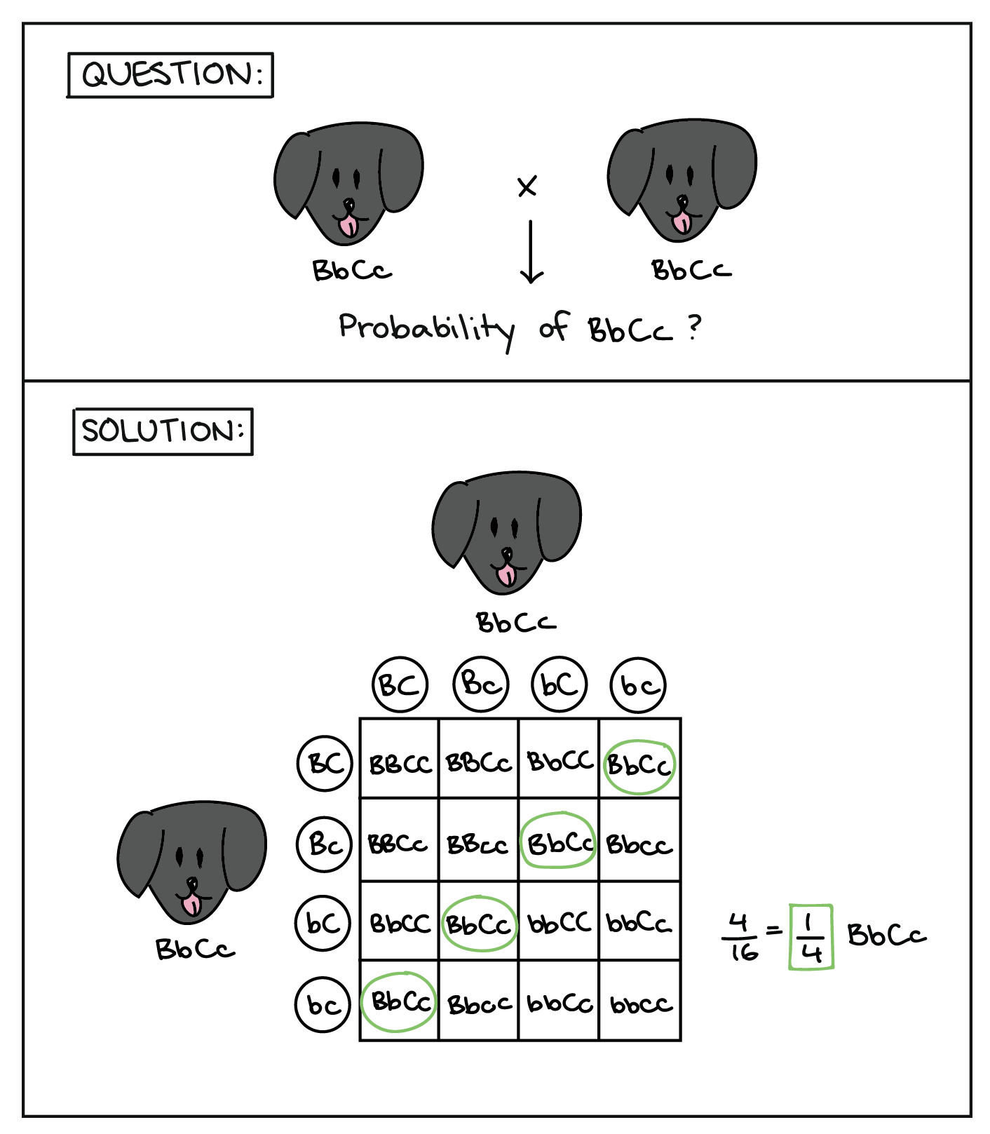
One approach is to draw a 16-square Punnett square. For a cross involving two genes, a Punnett square is still a good strategy. Alternatively, we can use a shortcut technique involving four-square Punnett squares and a little application of the product rule. In this technique, we break the overall question down into two smaller questions, each relating to a different genetic event:

1. What’s the probability of getting a Bb genotype?
2. What’s the probability of getting an Cc genotype?

In order for a puppy to have a BbCc genotype, both of these events must take place: the puppy must receive Bb alleles, and it must receive Cc alleles. The two events are independent because the genes assort independently (don't affect one another's inheritance). So, once we calculate the probability of each genetic event, we can multiply these probabilities using the product rule to get the probability of the genotype of interest (BbCc).

To calculate the probability of getting a Bb genotype, we can draw a 4-square Punnett square using the parents' alleles for the coat color gene only, as shown above. Using the Punnett square, you can see that the probability of the Bb genotype is 1/2. (Alternatively, we could have calculated the probability of Bb using the product rule for gamete contributions from the two parents and the sum rule for the two gamete combinations that give Bb.) Using a similar Punnett square for the parents' fur texture alleles, the probability of getting an Cc genotype is also 1/2. To get the overall probability of the BbCc genotype, we can simply multiply the two probabilities, giving an overall probability of 1/4.

[Let's check that with a Punnett square]

You can also use this technique to predict phenotype frequencies. Give it a try in the practice question below!

Check your understanding

Query \(\PageIndex{1}\)

[Hint]

We can break the question down into two smaller questions:

1. What fraction of offspring will have black coat color?
2. What fraction of offspring will have straight fur?

Since black coat color and straight fur are dominant traits, all BB and Bb puppies will have black coats, and all CC and Cc puppies will have straight fur, corresponding to 3/4 of puppies in each case. (You can draw out the individual Punnett squares for the color and texture genes to confirm these frequencies.)

To get the probability of a puppy having both black coat color and straight fur, you can multiply the probabilities of these two independent events: \((3/4)\cdot(3/4)=9/16\).

9/16 of the puppies will have black coats and straight fur.

Beyond dihybrid crosses

The probability method is most powerful (and helpful) in cases involving a large number of genes.

For instance, imagine a cross between two individuals with various alleles of four unlinked genes: AaBbCCdd x AabbCcDd. Suppose you wanted to figure out the probability of getting offspring with the dominant phenotype for all four traits. Fortunately, you can apply the exact same logic as in the case of the dihybrid crosses above. To have the dominant phenotype for all four traits, and organism must have: one or more copies of the dominant allele A and one or more copies of dominant allele B and one or more copies of the dominant allele C and one or more copies of the dominant allele D.

Since the genes are unlinked, these are four independent events, so we can calculate a probability for each and then multiply the probabilities to get the probability of the overall outcome.

• The probability of getting one or more copies of the dominant A allele is 3/4. (Draw a Punnett square for Aa x Aa to confirm for yourself that 3 out of the 4 squares are either AA or Aa.)
• The probability of getting one or more copies of the dominant B allele is 1/2. (Draw a Punnett square for Bb x bb: you’ll find that half the offspring are Bb, and the other half bb.)
• The probability of getting one or more copies of the dominant C allele is 1. (If one of the parents is homozygous CC, there’s no way to get offspring without a C allele!)
• The probability of getting one or more copies of the dominant D allele is 1/2, as for B. (Half the offspring will be Dd, and the other half will be dd.)

To get the overall probability of offspring with the dominant phenotype for all four genes, we can multiply the probabilities of the four independent events: \((3/4)\cdot(1/2)\cdot(1)\cdot(1/2)=3/16\).

Check your understanding

Query \(\PageIndex{2}\)

[Hint]

It’s not possible to get a quadruple homozygous recessive individual out of this cross. That’s because the probability of getting two recessive c alleles is zero. The first parent has only dominant alleles for this gene, ensuring that each of the offspring will receive at least one dominant C allele (and thus cannot display the recessive phenotype).

How does the zero probability of a cc genotype figure in mathematically? To get the overall probability of the aabbccdd genotype, we'd have to multiply the probabilities of the desired genotypes for the other three genes (aa, 1/4; bb, 1/2; and dd, 1/2) by the zero corresponding to the cc genotype, giving an overall probability of zero.

\(P(aabbccdd)=P(aa) \cdot P(bb) \cdot P(cc) \cdot P(dd)\)

\(P(aabbccdd)=(1/4)\cdot(1/2)\cdot(0)\cdot(1/2)=0\)

The probability of getting an individual with a recessive phenotype for all four genes is 0.

Contributors and Attributions

• Khan Academy (CC BY-NC-SA 3.0; All Khan Academy content is available for free at www.khanacademy.org)

[Attribution and references]

Attribution:

This article is a modified derivative of the following articles:

• “Mendel’s experiments and the laws of probability,” by OpenStax College, Biology (CC BY 3.0). Download the original article for free at http://cnx.org/contents/185cbf87-c72e-48f5-b51e-f14f21b5eabd@9.85.
• “Laws of inheritance,” by OpenStax College, Biology (CC BY 3.0). Download the original article for free at http://cnx.org/contents/185cbf87-c72e-48f5-b51e-f14f21b5eabd@9.85.

The modified article is licensed under a CC BY-NC-SA 4.0 license.

Additional references:

Griffiths, A. J. F., Miller, J. H., Suzuki, D. T., Lewontin, R. C., and Gelbart, W. M. (2000). Using genetic ratios. In An introduction to genetic analysis (7th ed.). New York, NY: W. H. Freeman. Retrieved from http://www.ncbi.nlm.nih.gov/books/NBK21812/.

Purves, W. K., Sadava, D., Orians, G. H., and Heller, H. C. (2003). Punnett squares or probability calculations: A choice of methods. In Life: The science of biology (7th ed., pp. 195-196). Sunderland, MA: Sinauer Associates.

Reece, J. B., Urry, L. A., Cain, M. L., Wasserman, S. A., Minorsky, P. V., and Jackson, R. B. (2011). Mendel and the gene idea. In Campbell Biology (10th ed., pp. 267-291). San Francisco, CA: Pearson.

Raven, P. H., Johnson, G. B., Mason, K. A., Losos, J. B., and Singer, S. R. (2014). Patterns of inheritance. In Biology (10th ed., AP ed., pp. 221-238). New York, NY: McGraw-Hill.

Staroscik, A. (2015). Punnett square calculator. In SciencePrimer.com. Retrieved from http://scienceprimer.com/punnett-square-calculator.

The Adapa Project. (2014, August 13). What are the laws of segregation and independent assortment and why are they so important? InBioBook. Retrieved from https://adapaproject.org/bbk_temp/tiki-index.php?page=Leaf%3A+What+are+the+laws+of+segregation+and+independent+assortment+and+why+are+they+so+important%3F.