
6.3: Variation in rates of trait evolution across clades


( \newcommand{\kernel}{\mathrm{null}\,}\)
One assumption of Brownian motion is that the rate of change (σ2) is constant, both through time and across lineages. However, some of the most interesting hypotheses in evolution relate to differences in the rates of character change across clades. For example, key innovations are evolutionary events that open up new areas of niche space to evolving clades (Hunter 1998; reviewed in Alfaro 2013). This new niche space is an ecological opportunity that can then be filled by newly evolved species (Yoder et al. 2010). If this were happening in a clade, we might expect that rates of trait evolution would be elevated following the acquisition of the key innovation (Yoder et al. 2010).
There are several methods that one can use to test for differences in the rate of evolution across clades. First, one can compare the magnitude of independent contrasts across clades; second, one can use model comparison approaches to compare the fit of single- and multiple-rate models to data on trees; and third, one can use a Bayesian approach combined with reversible-jump machinery to try to find the places on the tree where rate shifts have occurred. I will explain each of these methods in turn.
Rate tests using phylogenetic independent contrasts
One of the earliest methods developed to compare rates across clades is to compare the magnitude of independent contrasts calculated in each clade (e.g. Garland 1992). To do this, one first calculates standardized independent contrasts, separating those contrasts that are calculated within each clade of interest. As we noted in Chapter 5, these contrasts have arbitrary sign (positive or negative) but if they are squared, represent independent estimates of the Brownian motion rate parameter (σ2). Basically, when rates of evolution are high, we should see large independent contrasts in that part of the tree (Garland 1992).
In his original description of this approach, Garland (1992) proposed using a statistical test to compare the absolute value of contrasts between clades (or between a single clade and the rest of the phylogenetic tree). In particular, Garland (1992) suggests using a t-test, as long as the absolute value of independent contrasts are approximately normally distributed. However, under a Brownian motion model, the contrasts themselves – but not the absolute values of the contrasts – should be approximately normal, so it is quite likely that absolute values of contrasts will strongly violate the assumptions of a t-test.
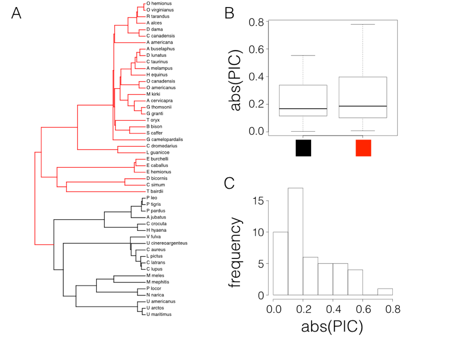
In fact, if we try this test on mammal body size, contrasting the two major clades in the tree (carnivores versus non-carnivores, Figure 6.2A), there looks to be a small difference in the absolute value of contrasts (Figure 6.2B). A t-test is not significant (Welch two-sample t-test P = 0.42), but we also can see that the distribution of PIC absolute values is strongly skewed (Figure 6.2C).
There are other simple options that might work better in general. For example, one could also compare the magnitudes of the squared contrasts, although these are also not expected to follow a normal distribution. Alternatively, we can again follow Garland’s (1992) suggestion and use a Mann-Whitney U-test, the nonparametric equivalent of a t-test, on the absolute values of the contrasts. Since Mann-Whitney U tests use ranks instead of values, this approach will not be sensitive to the fact that the absolute values of contrasts are not normal. If the P-value is significant for this test then we have evidence that the rate of evolution is greater in one part of the tree than another.
In the case of mammals, a Mann-Whitney U test also shows no significant differences in rates of evolution between carnivores and other mammals (W = 251, P = 0.70).
Rate tests using maximum likelihood and AIC
One can also carry out rate comparisons using a model-selection framework (O’Meara et al. 2006; Thomas et al. 2006). To do this, we can fit single- and multiple-rate Brownian motion models to a phylogenetic tree, then compare them using a model selection method like AICc. For example, in the example above, we tested whether or not one subclade in the mammal tree (carnivores) has a very different rate of body size evolution than the rest of the clade. We can use an ML-based model selection method to compare the fit of a single-rate model to a model where the evolutionary rate in carnivores is different from the rest of the clade, and use this test evaluate the support for that hypothesis.
This test requires the likelihood for a multi-rate Brownian motion model on a phylogenetic tree. We can derive such an equation following the approach presented in Chapter 4. Recall that the likelihood equations for (constant-rate) Brownian motion use a phylogenetic variance-covariance matrix, C, that is based on the branch lengths and topology of the tree. For single-rate Brownian motion, the elements in C are derived from the branch lengths in the tree. Traits are drawn from a multivariate normal distribution with variance-covariance matrix:
VH1 = σ2Ctree
One simple way to fit a multi-rate Brownian motion model is to construct separate C matrices, one for each rate category in the tree. For example, imagine that most of a clade evolves under a Brownian motion model with rate σ12, but one clade in the tree evolves at a different (higher or lower) rate, σ22. One can construct two C matrices: the first matrix, C1, includes branches that evolve under rate σ12, while the second, C2, includes only branches that evolve under rate σ22. Since all branches in the tree are included in one of these two categories, it will be true that Ctree = C1 + C2. For any particular values of these two rates, traits are drawn from a multivariate normal distribution with variance-covariance matrix:
VH2 = σ21C1 + σ22C2
We can now treat this as a model comparison-problem, contrasting H1: traits on the tree evolved under a constant-rate Brownian motion model, with H2: traits on the tree evolved under a multi-rate Brownian motion model. Note that H1 is a special case of H2 when σ12 = σ22; that is, these two models are nested and can be compared using a likelihood ratio test. Of course, one can also compare the two models using AICc.
For the mammal body size example, you might recall our ML single-rate Brownian motion model (σ2 = 0.088, ˉz(0)=4.64, lnL = −78.0, AICc = 160.4). We can compare that to the fit of a model where carnivores get their own rate parameter (σc2) that might differ from that of the rest of the tree (σo2). Fitting that model, we find the following maximum likelihood parameter estimates: ˆσ2c=0.068, ˆσ2o=0.01, ˆˉz(0)=4.51). Carnivores do appear to be evolving more rapidly. However, the fit of this model is not substantially better than the single-rate Brownian motion (lnL = −77.6, AICc = 162.3).
There is one complication, which is how to deal with the actual branch along which the rate shift is thought to have occurred. O’Meara et al. (2006) describe “censored” and “noncensored” versions of their test, which differ in whether or not branches where rate shifts actually occur are included in the calculation. In the censored version of the test, O’Meara et al. (2006) omit the branch where we think a shift occurred, while in the noncensored version O’Meara et al. (2006) include that branch in one of the two rate categories (this is what I did in the example above, adding the stem branch of carnivores in the “non-carnivore” category). One could also specify where, exactly, the rate shift occurred along the branch in question, placing part of the branch in each of the two rate categories as appropriate. However, since we typically have little information about what happened on particular branches in a phylogenetic tree, results from these two approaches are not very different – unless, as stated by O’Meara et al. (2006), unusual evolutionary processes have occurred on the branch in question.
A similar approach was described by Thomas et al. (2006) but considers differences across clades to include changes in any of the two parameters of a Brownian motion model (σ2, ˉz(0), or both). Remember that ˉz(0) is the expected mean of species within a clade under a Brownian motion, but also represents the starting value of the trait at time zero. Allowing ˉz(0) to vary across clades effectively allows different clades to have different “starting points” in phenotype space. In the case of comparing a monophyletic subclade to the rest of a tree, Thomas et al.’s (2006) approach is equivalent to the “censored” test described above. However, one drawback to both the Thomas et al. (2006) approach and the “censored” test is that, because clades each have their own mean, we no longer can tie the model that we fit using likelihood to any particular evolutionary process. Mathematically, changing ˉz(0) in a subclade postulates that the trait value changed somehow along the branch leading to that clade, but we do not specify the way that the trait changed – the change could have been gradual or instantaneous, and no amount or pattern of change is more or less likely than anything else. Of course, one can describe evolutionary scenarios that might act like this process - but we begin to lose any potential tie to explicit evolutionary processes.
Rate tests using Bayesian MCMC
It is also possible to carry out this test in a Bayesian MCMC framework. The simplest way to do that would be to fit model H2 above, that traits on the tree evolved under a multi-rate Brownian motion model, in a Bayesian framework. We can then specify prior distributions and sample the three model parameters (ˉz(0), σ12, and σ22) through our MCMC. At the end of our analysis, we will have posterior distributions for the three model parameters. We can test whether rates differ among clades by calculating a posterior distribution for the composite parameter σdiff2 = σ12 − σ22. The proportion of the posterior distribution for σdiff2 that is positive or negative gives the posterior probability that σ12 is greater or less than σ22, respectively.
Perhaps, though, researchers are unsure of where, exactly, the rate shift might have occurred, and want to incorporate some uncertainty in their analysis. In some cases, rate shifts are thought to be associated with some other discrete character, such as living on land (state 0) or in the water (1). In such cases, one way to proceed is to use stochastic character mapping (see Chapter 8) to map state changes for the discrete character on the tree, and then run an analysis where rates of evolution of the continuous character of interest depend on the mapping of our discrete states. This protocol is described most fully by Revell (2013), who also points out that rate estimates are biased to be more similar when the discrete character evolves quickly.
It is even possible to explore variation in Brownian rates without invoking particular a priori hypotheses about where the rates might change along branches in a tree. These methods rely on reversible-jump MCMC, a Bayesian statistical technique that allows one to consider a large number of models, all with different numbers of parameters, in a single Bayesian analysis. In this case, we consider models where each branch in the tree can potentially have its own Brownian rate parameter. By constraining sets of these rate parameters to be equal to one another, we can specify a huge number of models for rate variation across trees. The reversible-jump machinery, which is beyond the scope of this book, allows us to generate a posterior distribution that spans this large set of models where rates vary along branches in a phylogenetic tree (see Eastman et al. 2011 for details).