6.2: Transforming the evolutionary variance-covariance matrix

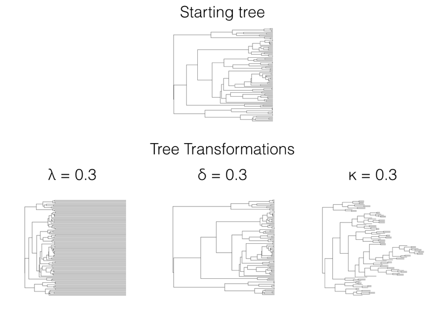
In 1999, Mark Pagel introduced three statistical models that allow one to test whether data deviates from a constant-rate process evolving on a phylogenetic tree (Pagel 1999a,b)¹. Each of these three models is a statistical transformation of the elements of the phylogenetic variance-covariance matrix, C, that we first encountered in Chapter 3. All three can also be thought of as a transformation of the branch lengths of the tree, which adds a more intuitive understanding of the statistical properties of the tree transformations (Figure 6.1). We can transform the tree and then simulate characters under a Brownian motion model on the transformed tree, generating very different patterns than if they had been simulated on the starting tree.

Figure 6.1. Branch length transformations effectively alter the relative rate of evolution on certain branches in the tree. If we make a branch longer, there is more “evolutionary time” for characters to change, and so we are effectively increasing the rate of evolution along that branch. Image by the author, can be reused under a CC-BY-4.0 license.

There are three Pagel tree transformations (lambda: λ, delta: δ, and kappa: κ). I will describe each of them along with common methods for fitting Pagel models under ML, AIC, and Bayesian frameworks. Pagel’s three transformations can also be related to evolutionary processes, although those relationships are sometimes vague compared to approaches based on explicit evolutionary models rather than tree transformations (see below for more comments on this distinction).

Perhaps the most commonly used Pagel tree transformation is λ. When using λ, one multiplies all off-diagonal elements in the phylogenetic variance-covariance matrix by the value of λ, restricted to values of 0 ≤ λ ≤ 1. The diagonal elements remain unchanged. So, if the original matrix for r species is:

\[ \mathbf{C_o} = \begin{bmatrix} \sigma_1^2 & \sigma_{12} & \dots & \sigma_{1r}\\ \sigma_{21} & \sigma_2^2 & \dots & \sigma_{2r}\\ \vdots & \vdots & \ddots & \vdots\\ \sigma_{r1} & \sigma_{r2} & \dots & \sigma_{r}^2\\ \end{bmatrix} \label{6.1}\]

Then the transformed matrix will be:

\[ \mathbf{C_\lambda} = \begin{bmatrix} \sigma_1^2 & \lambda \cdot \sigma_{12} & \dots & \lambda \cdot \sigma_{1r}\\ \lambda \cdot \sigma_{21} & \sigma_2^2 & \dots & \lambda \cdot \sigma_{2r}\\ \vdots & \vdots & \ddots & \vdots\\ \lambda \cdot \sigma_{r1} & \lambda \cdot \sigma_{r2} & \dots & \sigma_{r}^2\\ \end{bmatrix} \label{6.2}\]

In terms of branch length transformations, λ compresses internal branches while leaving the tip branches of the tree unaffected (Figure 6.1). λ can range from 1 (no transformation) to 0 (which results in a complete star phylogeny, with all tip branches equal in length and all internal branches of length 0). One can in principle use some values of λ greater than one on most variance-covariance matrices, although many values of λ > 1 result in matrices that are not valid variance-covariance matrices and/or do not correspond with any phylogenetic tree transformation. For this reason I recommend that λ be limited to values between 0 and 1.

λ is often used to measure the “phylogenetic signal” in comparative data. This makes intuitive sense, as λ scales the tree between a constant-rates model (λ = 1) to one where every species is statistically independent of every other species in the tree (λ = 0). Statistically, this can be very useful information. However, there is some danger is in attributing a statistical result – either phylogenetic signal or not – to any particular biological process. For example, phylogenetic signal is sometimes called a “phylogenetic constraint.” But one way to obtain a high phylogenetic signal (λ near 1) is to evolve traits under a Brownian motion model, which involves completely unconstrained character evolution. Likewise, a lack of phylogenetic signal – which might be called “low phylogenetic constraint” – results from an OU model with a high α parameter (see below), which is a model where trait evolution away from the optimal value is, in fact, highly constrained. Revell et al. (2008) show a broad range of circumstances that can lead to patterns of high or low phylogenetic signal, and caution against over-interpretation of results from analyses of phylogenetic signal, like Pagel’s λ. Also worth noting is that statistical estimates of λ under a ML model tend to be clustered near 0 and 1 regardless of the true value, and AIC model selection can tend to prefer models with λ ≠ 0 even when data is simulated under Brownian motion (Boettiger et al. 2012).

Pagel’s δ is designed to capture variation in rates of evolution through time. Under the δ transformation, all elements of the phylogenetic variance-covariance matrix are raised to the power δ, assumed to be positive. So, if our original C matrix is given above (equation 6.1), then the δ-transformed version will be:

\[ \mathbf{C_\delta} = \begin{bmatrix} (\sigma_1^2)^\delta & (\sigma_{12})^\delta & \dots & (\sigma_{1r})^\delta\\ (\sigma_{21})^\delta & (\sigma_2^2)^\delta & \dots & (\sigma_{2r})^\delta\\ \vdots & \vdots & \ddots & \vdots\\ (\sigma_{r1})^\delta & (\sigma_{r2})^\delta & \dots & (\sigma_{r}^2)^\delta\\ \end{bmatrix} \label{6.3} \]

Since these elements represent the heights of nodes in the phylogenetic tree, then δ can also be viewed as a transformation of phylogenetic node heights. When δ is one, the tree is unchanged and one still has a constant-rate Brownian motion process; when δ is less than 1, node heights are reduced, but deeper branches in the tree are reduced less than shallower branches (Figure 6.1). This effectively represents a model where the rate of evolution slows through time. By contrast, δ > 1 stretches the shallower branches in the tree more than the deep branches, mimicking a model where the rate of evolution speeds up through time. There is a close connection between the δ model, the ACDC model (Blomberg et al. 2003), and Harmon et al.’s (2010) early burst model [see also Uyeda and Harmon (2014), especially the appendix).

Finally, the κ transformation is sometimes used to capture patterns of “speciational” change in trees. In the κ model, one raises all of the branch lengths in the tree by the power κ (we require that κ ≥ 0). This has a complicated effect on the phylogenetic variance-covariance matrix, as the effect that this transformation has on each covariance element depends on both the value of κ and the number of branches that extend from the root of the tree to the most recent common ancestor of each pair of species. So, if our original C matrix is given by Equation \ref{6.1}, the transformed version will be:

\[ \begin{array}{l} \mathbf{C_o} = \\ \left(\begin{smallmatrix} b_{1,1}^k + b_{1,2}^k \dots + b_{1,d_1}^k & b_{1-2,1}^k + b_{1-2,2}^k \dots + b_{1-2,d_{1-2}}^k & \dots & b_{1-r,1}^k + b_{1-r,2}^k \dots + b_{1-r,d_{1-r}}^k \\ b_{2-1,1}^k + b_{2-1,2}^k \dots + b_{2-1,d_{1-2}}^k & b_{2,1}^k + b_{2,2}^k \dots + b_{2,d_2}^k & \dots & b_{2-r,1}^k + b_{2-r,2}^k \dots + b_{2-r,d_{2-r}}^k \\ \vdots & \vdots & \ddots & \vdots\\ b_{r-1,1}^k + b_{r-1,2}^k \dots + b_{r-1,d_{1-r}}^k & b_{r-2,1}^k + b_{r-2,2}^k \dots + b_{r-2,d_{1-2}}^k & \dots & b_{r,1}^k + b_{r,2}^k \dots + b_{r,d_{r}}^k \\ \end{smallmatrix}\right) \\ \end{array} \label{6.4} \]

where b_x, y is the branch length of the branch that is the most recent common ancestor of taxa x and y, while d_x, y is the total number of branches that one encounters traversing the path from the root to the most recent common ancestor of the species pair specified by x, y (or to the tip x if just one taxon is specified). Needless to say, this transformation is easier to understand as a transformation of the tree branches themselves rather than of the associated variance-covariance matrix.

When the κ parameter is one, the tree is unchanged and one still has a constant-rate Brownian motion process; when κ = 0, all branch lengths are one. κ values in between these two extremes represent intermediates (Figure 6.1). κ is often interpreted in terms of a model where character change is more or less concentrated at speciation events. For this interpretation to be valid, we have to assume that the phylogenetic tree, as given, includes all (or even most) of the speciation events in the history of the clade. The problem with this assumption is that speciation events are almost certainly missing due to sampling: perhaps some living species from the clade have not been sampled, or species that are part of the clade have gone extinct before the present day and are thus not sampled. There are much better ways of estimating speciational models that can account for these issues in sampling (e.g. Bokma 2008; Goldberg and Igić 2012); these newer methods should be preferred over Pagel’s κ for testing for a speciational pattern in trait data.

There are two main ways to assess the fit of the three Pagel-style models to data. First, one can use ML to estimate parameters and likelihood ratio tests (or AIC_c scores) to compare the fit of various models. Each represents a three parameter model: one additional parameter added to the two parameters already needed to describe single-rate Brownian motion. As mentioned above, simulation studies suggest that this can sometimes lead to overconfidence, at least for the λ model. Sometimes researchers will compare the fit of a particular model (e.g. λ) with models where that parameter is fixed at its two extreme values (0 or 1; this is not possible with δ). Second, one can use Bayesian methods to estimate posterior distributions of parameter values, then inspect those distributions to see if they overlap with values of interest (say, 0 or 1).

We can apply these three Pagel models to the mammal body size data discussed in chapter 5, comparing the AIC_c scores for Brownian motion to that from the three transformations. We obtain the following results:

Model	Parameter estimates	lnL	AICc
Brownian motion	σ^2 = 0.088, θ = 4.64	-78.0	160.4
lambda	σ^2 = 0.085, θ = 4.64, λ = 1.0	-78.0	162.6
delta	σ^2 = 0.063, θ = 4.60, δ = 1.5	-77.7	162.0
kappa	σ^2 = 0.170, θ = 4.64, κ = 0.66	-77.3	161.1

Note that Brownian motion is the preferred model with the lowest AIC_c score, but also that all four AIC_c scores are within 3 units – meaning that we cannot easily distinguish among them using our mammal data.