
10.4: A phase space example
- Page ID
- 25480

\( \newcommand{\vecs}[1]{\overset { \scriptstyle \rightharpoonup} {\mathbf{#1}} } \)
\( \newcommand{\vecd}[1]{\overset{-\!-\!\rightharpoonup}{\vphantom{a}\smash {#1}}} \)
\( \newcommand{\id}{\mathrm{id}}\) \( \newcommand{\Span}{\mathrm{span}}\)
( \newcommand{\kernel}{\mathrm{null}\,}\) \( \newcommand{\range}{\mathrm{range}\,}\)
\( \newcommand{\RealPart}{\mathrm{Re}}\) \( \newcommand{\ImaginaryPart}{\mathrm{Im}}\)
\( \newcommand{\Argument}{\mathrm{Arg}}\) \( \newcommand{\norm}[1]{\| #1 \|}\)
\( \newcommand{\inner}[2]{\langle #1, #2 \rangle}\)
\( \newcommand{\Span}{\mathrm{span}}\)
\( \newcommand{\id}{\mathrm{id}}\)
\( \newcommand{\Span}{\mathrm{span}}\)
\( \newcommand{\kernel}{\mathrm{null}\,}\)
\( \newcommand{\range}{\mathrm{range}\,}\)
\( \newcommand{\RealPart}{\mathrm{Re}}\)
\( \newcommand{\ImaginaryPart}{\mathrm{Im}}\)
\( \newcommand{\Argument}{\mathrm{Arg}}\)
\( \newcommand{\norm}[1]{\| #1 \|}\)
\( \newcommand{\inner}[2]{\langle #1, #2 \rangle}\)
\( \newcommand{\Span}{\mathrm{span}}\) \( \newcommand{\AA}{\unicode[.8,0]{x212B}}\)
\( \newcommand{\vectorA}[1]{\vec{#1}} % arrow\)
\( \newcommand{\vectorAt}[1]{\vec{\text{#1}}} % arrow\)
\( \newcommand{\vectorB}[1]{\overset { \scriptstyle \rightharpoonup} {\mathbf{#1}} } \)
\( \newcommand{\vectorC}[1]{\textbf{#1}} \)
\( \newcommand{\vectorD}[1]{\overrightarrow{#1}} \)
\( \newcommand{\vectorDt}[1]{\overrightarrow{\text{#1}}} \)
\( \newcommand{\vectE}[1]{\overset{-\!-\!\rightharpoonup}{\vphantom{a}\smash{\mathbf {#1}}}} \)
\( \newcommand{\vecs}[1]{\overset { \scriptstyle \rightharpoonup} {\mathbf{#1}} } \)
\( \newcommand{\vecd}[1]{\overset{-\!-\!\rightharpoonup}{\vphantom{a}\smash {#1}}} \)
\(\newcommand{\avec}{\mathbf a}\) \(\newcommand{\bvec}{\mathbf b}\) \(\newcommand{\cvec}{\mathbf c}\) \(\newcommand{\dvec}{\mathbf d}\) \(\newcommand{\dtil}{\widetilde{\mathbf d}}\) \(\newcommand{\evec}{\mathbf e}\) \(\newcommand{\fvec}{\mathbf f}\) \(\newcommand{\nvec}{\mathbf n}\) \(\newcommand{\pvec}{\mathbf p}\) \(\newcommand{\qvec}{\mathbf q}\) \(\newcommand{\svec}{\mathbf s}\) \(\newcommand{\tvec}{\mathbf t}\) \(\newcommand{\uvec}{\mathbf u}\) \(\newcommand{\vvec}{\mathbf v}\) \(\newcommand{\wvec}{\mathbf w}\) \(\newcommand{\xvec}{\mathbf x}\) \(\newcommand{\yvec}{\mathbf y}\) \(\newcommand{\zvec}{\mathbf z}\) \(\newcommand{\rvec}{\mathbf r}\) \(\newcommand{\mvec}{\mathbf m}\) \(\newcommand{\zerovec}{\mathbf 0}\) \(\newcommand{\onevec}{\mathbf 1}\) \(\newcommand{\real}{\mathbb R}\) \(\newcommand{\twovec}[2]{\left[\begin{array}{r}#1 \\ #2 \end{array}\right]}\) \(\newcommand{\ctwovec}[2]{\left[\begin{array}{c}#1 \\ #2 \end{array}\right]}\) \(\newcommand{\threevec}[3]{\left[\begin{array}{r}#1 \\ #2 \\ #3 \end{array}\right]}\) \(\newcommand{\cthreevec}[3]{\left[\begin{array}{c}#1 \\ #2 \\ #3 \end{array}\right]}\) \(\newcommand{\fourvec}[4]{\left[\begin{array}{r}#1 \\ #2 \\ #3 \\ #4 \end{array}\right]}\) \(\newcommand{\cfourvec}[4]{\left[\begin{array}{c}#1 \\ #2 \\ #3 \\ #4 \end{array}\right]}\) \(\newcommand{\fivevec}[5]{\left[\begin{array}{r}#1 \\ #2 \\ #3 \\ #4 \\ #5 \\ \end{array}\right]}\) \(\newcommand{\cfivevec}[5]{\left[\begin{array}{c}#1 \\ #2 \\ #3 \\ #4 \\ #5 \\ \end{array}\right]}\) \(\newcommand{\mattwo}[4]{\left[\begin{array}{rr}#1 \amp #2 \\ #3 \amp #4 \\ \end{array}\right]}\) \(\newcommand{\laspan}[1]{\text{Span}\{#1\}}\) \(\newcommand{\bcal}{\cal B}\) \(\newcommand{\ccal}{\cal C}\) \(\newcommand{\scal}{\cal S}\) \(\newcommand{\wcal}{\cal W}\) \(\newcommand{\ecal}{\cal E}\) \(\newcommand{\coords}[2]{\left\{#1\right\}_{#2}}\) \(\newcommand{\gray}[1]{\color{gray}{#1}}\) \(\newcommand{\lgray}[1]{\color{lightgray}{#1}}\) \(\newcommand{\rank}{\operatorname{rank}}\) \(\newcommand{\row}{\text{Row}}\) \(\newcommand{\col}{\text{Col}}\) \(\renewcommand{\row}{\text{Row}}\) \(\newcommand{\nul}{\text{Nul}}\) \(\newcommand{\var}{\text{Var}}\) \(\newcommand{\corr}{\text{corr}}\) \(\newcommand{\len}[1]{\left|#1\right|}\) \(\newcommand{\bbar}{\overline{\bvec}}\) \(\newcommand{\bhat}{\widehat{\bvec}}\) \(\newcommand{\bperp}{\bvec^\perp}\) \(\newcommand{\xhat}{\widehat{\xvec}}\) \(\newcommand{\vhat}{\widehat{\vvec}}\) \(\newcommand{\uhat}{\widehat{\uvec}}\) \(\newcommand{\what}{\widehat{\wvec}}\) \(\newcommand{\Sighat}{\widehat{\Sigma}}\) \(\newcommand{\lt}{<}\) \(\newcommand{\gt}{>}\) \(\newcommand{\amp}{&}\) \(\definecolor{fillinmathshade}{gray}{0.9}\)For an example of finding equilibria and stability, consider two competing species with intrinsic growth rates r1 = 1.2 and r2 = 0.8. Let each species inhibit itself in such a way that s1,1 =−1 and s2,2 =−1, let Species 2 inhibit Species 1 more strongly than it inhibits itself, with s1,2 =−1.2, and let Species 1 inhibit Species 2 less strongly than it inhibits itself, with s2,1 =−0.5. These conditions are summarized in Box 10.2.2 for reference. The question is, what are the equilibria in this particular competitive system, and what will their stability be?
First, there is an equilibrium at the origin (0,0) in these systems, where both species are extinct. This is sometimes called the “trivial equilibrium,” and it may or may not be stable. From Table 10.2.1, the eigenvalues of the equilibrium at the origin are r1 and r2 —in this case 1.2 and 0.8. These are both positive, so from the rules for eigenvalues in Box 10.2.1, the equilibrium at the origin in this case is unstable. If no individuals of either species exist in an area, none will arise. But if any individuals of either species somehow arrive in the area, or if both species arrive, the population will increase. This equilibrium is thus unstable. It is shown in the phase space diagram of Figure \(\PageIndex{1}\), along with the other equilibria in the system.
box \(\PageIndex{1}\) calculated results for the sample competitive system
| Equilibrium | Coordinates | Eigenvalues | Condition |
| Origin | (0,0) | (1.2,0.8) | Unstable |
| Horizontal axis | (1.2,0) | (-1.2,0.2) | Unstable |
| Vertical axis | (0,0.8) | (-0.8,0.24) | Unstable |
| Interior | (0.6,0.5) | (-0.123,-0.977) | Stable |
On the horizontal axis, where Species 2 is not present, the equilibrium of Species 1 is N'1 = −r1/s1,1 = 1.2. That is as expected—it is just like the equilibrium of N' = −r /s for a single species—because it indeed is a single species when Species 2 is not present. As to the stability, one eigenvalue is −r1, which is −1.2, which is negative, so it will not cause instability. For the other eigenvalue at this equilibrium, you need to calculate q from Table 10.2.1. You should get q =−0.2, and if you divide that by s1,1, you should get 0.2. This is positive, so by the rules of eigenvalues in Box 10.2.1, the equilibrium on the horizontal axis is unstable. Thus, if Species 1 is at its equilibrium and an increment of Species 2 arrives, Species 2 will increase and the equilibrium will be abandoned.
Likewise, on the vertical axis, where Species 1 is not present, the equilibrium of Species 2 is N2 = −r2/s2,2 = 0.8. Calculate the eigenvalues at this equilibrium from Table 10.2.1 and you should get p=−0.24, and dividing by s2,2 give eigenvalues of −0.8 and 0.24. With one negative and the other positive, by the rules of eigenvalues in Box 10.2.1 the equilibrium on the vertical axis is also unstable.
Finally, for the fourth equilibrium—the interior equilibirum where both species are present—calculate a, b, and c from the table. You should get a =−0.4, b =−0.44, and c=−0.048. Now the interior equilibrium is N'1 = p/a = 0.6 and N'2 = q/a = 0.5.
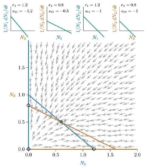
But is it stable? Notice the formula for the eigenvalues of the interior equilibrium in Table 10.2.1, in terms of a, b, and c. It is simply the quadratic formula! This is a clue that the eigenvalues are embedded in a quadratic equation, ax2 + bx + c = 0. And if you start a project to derive the formula for eigenvalues with pencil and paper, you will see that indeed they are. In any case, working it out more simply from the formula in the table, you should get −0.123 and −0.977. Both are negative, so by the rules of Box 10.2.1 the interior equilibrium for this set of parameters is stable.
As a final note, the presence of the square root in the formula suggests that eigenvalues can have imaginary parts, if the square root covers a negative number. The rules of eigenvalues in Box 10.2.1 still apply in this case, but only to the real part of the eigenvalues. Suppose, for example, that the eigenvalues are \(\frac{-1\pm\sqrt{-5}}{2}\,=\,-0..5\pm\,1.118i\). These would be stable because the real part, −0.5, is negative. But it turns out that because the imaginary part, \(\pm\,1.118i\), is not zero, the system would cycle around the equilibrium point, as predator–prey systems do.
In closing this part of the discussion, we should point out that eigenvectors and eigenvalues have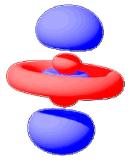 broad applications. They reveal, for instance, electron orbitals inside atoms (right), alignment of multiple variables in statistics, vibrational modes of piano strings, and rates of the spread of disease, and are used for a bounty of other applications. Asking how eigenvalues can be used is a bit like asking how the number seven can be used. Here, however, we simply employ them to evaluate the stability of equilibria.
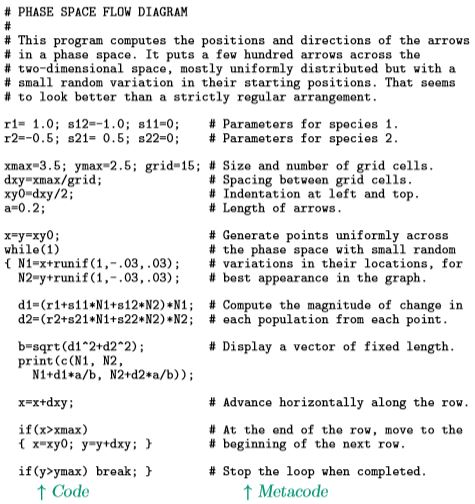
Program \(\PageIndex{1}\) Sample program in R to generate a phase space of arrows, displaying the locations of the beginning and ends of the arrows, which are passed through a graphics program for display. The ‘while(1)’ statement means “while forever”, and is just an easy way to keep looping until conditions at the bottom of the loop detect the end and break out.