26.2: Basics of Phylogeny

Trees

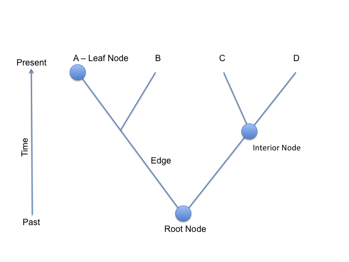
A tree is a mathematical representation of relationships between objects. A general tree is built from nodes and edges. Each node represents an object, and each edge represents a relationship between two nodes. In the case of phylogenetic trees, we represent evolution using trees. In this case, each node represents a divergence event between two ancestral lineages, the leaves denote the set of present objects and the root represents the common ancestor.

Figure 26.2: Defining tree terminology. A tree of branching nodes is depicted with leaves at the top and the root on the bottom. Time continues upward, toward the leaves.

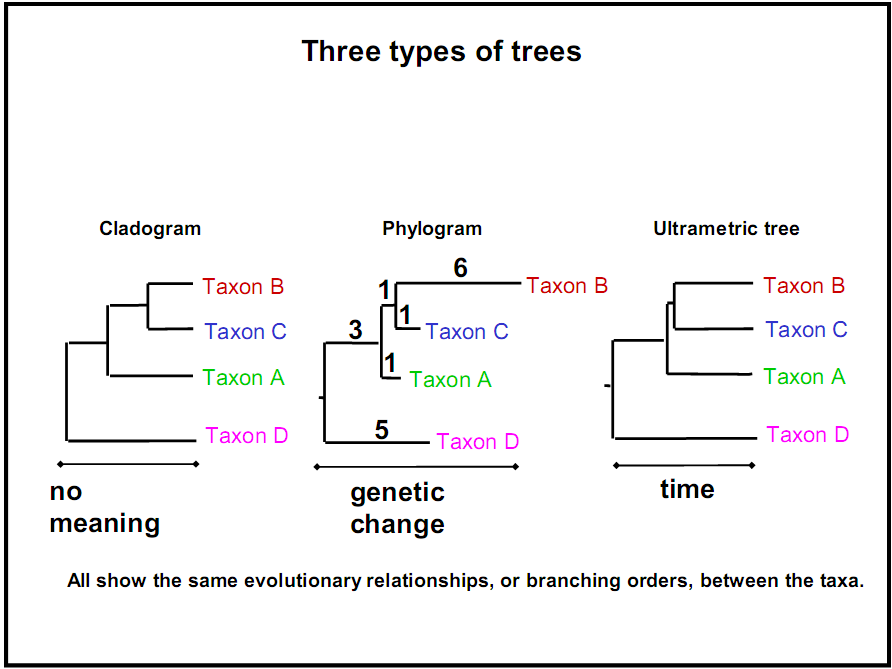
However, sometimes more information is reflected in the branch lengths, such as time elapsed or the amount of dissimilarity. According to these di↵erences, biological phylogenetic trees may be classified into three categories:

Cladogram: gives no meaning to branch lengths; only the sequence and topology of the branching matters.

Phylogram: Branch lengths are directly related to the amount of genetic change. The longer the branch of a tree, the greater the amount of phylogenetic change that has taken place. The leaves in this tree may not necessarily end on the same vertical line, due to different rates of mutation.

Chronogram (ultrametric tree): Branch lengths are directly related to time. The longer the branches of a tree, the greater the amount of time that has passed. The leaves in this tree necessarily end on the same vertical line (i.e. they are the same distance from the root), since they are all in the present unless extinct species were included in the tree. Although there is a correlation between branch lengths and genetic distance on a chronogram, they are not necessarily exactly proportional because evolution rates / mutation rates are not constant. Some species evolve and mutate faster than others, and some historical time periods foster faster rates of evolution than others.

Figure 26.3: Three types of trees.

A trait is any characteristic that an object or species possesses. In humans, an example of a trait may be bipedalism (the ability to walk upright) or the opposable thumb. Another human trait may be a specific DNA sequence that humans possess. The first examples of physical traits are called morphological traits, while the latter DNA traits are called sequence traits. Each has its advantages and disadvantages to study. All methods for tree-reconstruction rely on studying the occurrence of di↵erent traits in the given objects. In traditional phylogenetics the morphological data of different species were used for this purpose. In modern methods, genetic sequence data is used instead. Each has its advantages and disadvantages.

Morphological Traits: Arise from empirical evaluation of physical traits. This can be advantageous be- cause physical characteristics are very easy to quantify and understand for everyone, scientists and children alike. The disadvantages to this approach are that we can only evaluate a small set of traits, such as hair, nails, hoofs, teeth, etc. Further, these traits only allow us to build species. Finally, it is much easier to be ”tricked” by convergent evolution. Species that diverged millions of years ago may converge again on the few traits that are observable to scientists, giving a false representation of how closely related the species are.

Sequence Traits: Are discovered by studying the genomes of different species. This approach can be advantageous because it creates much more data and allows scientists to create gene trees in addition to species trees. The primary difficulty with this approach is that DNA is only built from 4 bases, so back mutations are frequent. In this approach, scientists must reconcile the signals of a large number of ill-behaved traits as opposed to that of a small number of well-behaved traits in the traditional approach. The rest of the chapter will focus principally on tree building from gene sequences.

Since this approach deals with comparing between pairs of genes, it is useful to understand the concept of homology: A pair of genes are called paralogues if they diverged from a duplication event, and orthologues if they diverged from a speciation event.

FAQ

Q: Would it be possible to use extinct species’ DNA sequences?

A: Current technologies only allow for usage of extant sequences. However, there have been a few successes in using extinct species’ DNA. DNA from frozen mammoths have been collected and are being sequences but due to DNA breaking down over time and contamination from the environment, it is very hard to extract correct sequences.

Once we have found genetic data for a set of species, we are interested in learning how those species relate to one another. Since we can, for the most part, only obtain DNA from living creatures, we must infer the existence of ancestors of each species, and ultimately infer the existence of a common ancestor. This is a challenging problem, because very limited data is available. The following sections will explore the modern methods for inferring ancestry from sequence data. They can be classified into two approaches, distance based methods and character based methods.

Distance based approaches take two steps to solve the problem, i.e. to quantify the amount of mutation that separates each pair of sequences (which may or may not be proportional to the time since they have been separated) and to fit the most likely tree according to the pair-wise distance matrix. The second step is usually a direct algorithm, based on some assumtions, but may be more complex.

Charecter based approaches instead try to find the tree that best explains the observed sequences. As opposed to direct reconstruction, these methods rely on tree proposal and scoring techniques to perform a heuristic search over the space of trees.

Did You Know?

Occam’s Razor, as discussed in previous chapters, does not always provide the most accurate hypothesis. In many cases during tree reconstruction, the simplest explanation is not the most probable. For example, a set of possible ancestries may be possible, given some observed data. In this case, the simplest ancestry may not be correct if a trait arose independently in two seperate lineages. This issue will be considered in a later section.