
26.3: Distance Based Methods
- Page ID
- 41080
The distance based models sequester the sequence data into pairwise distances. This step loses some information, but sets up the platform for direct tree reconstruction. The two steps of this method are hereby discussed in detail.
From alignment to distances
In order to understand how a distance-based model works, it is important to think about what distance means when comparing two sequences. There are three main interpretations.
Nucleotide Divergence is the idea of measuring distance between two sequences based on the number of places where nucleotides are not consistent. This assumes that evolution happens at a uniform rate across the genome, and that a given nucleotide is just as likely to evolve into any of the other three nucleotides. Although it has shortcomings, this is often a great way to think about it.
Transitions and Transversions This is similar to nucleotide divergence, but it recognizes that A-G and T-C substitutions are most frequent. Therefore, it keeps two parameters, the probability of a transition and the probability of a transversion.
Synonymous and non-synonymous substitutions This method keeps tracks of substitutions that affect the coded amino-acid by assuming that substitutions that do not change the coded protein will not be selected against, and will thus have a higher probability of occurring than those substitutions which do change the coded amino acid.
The naive way to interpret the separation between two sequences may be simply the number of mismatches, as described by nucleotide divergence above. While this does provide us a distance metric (i.e. d(a, b) + d(b, c) d(a, c)) this does not quite satisfy our requirements, because we want additive distances, i.e. those that satisfy d(a, b) + d(b, c) = d(a, c) for a path a ! b ! c of evolving sequence, because the amount of mutations accumulated along a path in the tree should be the sum of that of its individual components. However, the naive mismatch fraction do not always have this property, because this quantity is bounded by 1, while the sum of individual components can easily exceed 1.
The key to resolving this paradox is back-mutations. When a large number of mutations accumulate on a sequence, not all the mutations introduce new mismatches, some of them may occur on already mutated base pair, resulting in the mismatch score remaining the same or even decreasing. For small mismatch- scores however, this e↵ect is statistically insignificant, because there are vastly more identical pairs than mismatching pairs. However, for sequences separated by longer evolutionary distance, we must correct for this effect. The Jukes-Cantor model is one such simple markov model that takes this into account.
Jukes-Cantor distances
To illustrate this concept, consider a nucleotide in state ’A’ at time zero. At each time step, it has a probability 0.7 of retaining its previous state and probability 0.1 of transitioning to each of the other three states. The probability P(B|t) of observing state (base) B at time t essentially follows the recursion
\[P(B \mid t+1)=0.7 P(B \mid t)+0.1 \sum_{b \neq B} P(b \mid t)=0.1+0.6 P(B \mid t)\nonumber\]
Figure 26.5: Markov chain accounting for back mutations
If we plot P(B|t) versus t, we observe that the distribution starts o↵ as concentrated at the state ’A’ and gradually spreads over to the rest of the states, eventually going towards an equilibrium of equal probabilities. This progression makes sense, intuitively. Over millions of years, species can evolve so dramatically that they no longer resemble their ancestors. At that extreme, a given base location in the ancestor is just as likely to have evolved to any of the four possible bases in that location over time.
\[\begin{array}{lccccr}
\text { time:- } & 0 & 1 & 2 & 3 & 4 \\
\hline \text { A } & 1 & 0.7 & 0.52 & 0.412 & 0.3472 \\
\text { C } & 0 & 0.1 & 0.16 & 0.196 & 0.2196 \\
\text { G } & 0 & 0.1 & 0.16 & 0.196 & 0.2196 \\
\text { T } & 0 & 0.1 & 0.16 & 0.196 & 0.2196
\end{array}\nonumber\]
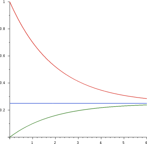
The essence of the Jukes Cantor model is to backtrack t, the amount of time elapsed from the fraction of altered bases. Conceptually, this is just inverting the x and y axis of the green curve. To model this quantitatively, we consider the following matrix S(t) which denotes the respective probabilities P(x|y,t) of observing base x given a starting state of base y in time \(\Delta\)t.
\[S(\Delta t)=\left(\begin{array}{cccc}
P(A \mid A, \Delta t) & P(A \mid G, \Delta t) & \cdots & P(A \mid T, \Delta t) \\
P(G \mid A, \Delta t) & \cdots & & \cdots \\
\cdots & & & \cdots \\
P(T \mid A, \Delta t) & \cdots & \cdots & P(T \mid T \Delta T)
\end{array}\right)\nonumber\]
We can assume this is a stationary markov model, implying this matrix is multiplicative, i.e.
\[S\left(t_{1}+t_{2}\right)=S\left(t_{1}\right) S\left(t_{2}\right)\]
For a very short time \(\epsilon\), we can assume that there is no second order effect, i.e. there isn’t enough time for two mutations to occur at the same nucleotide. So the probabilities of cross transitions are all proportional to \(\epsilon\). Further, in Jukes Cantor model, we assume that all the transition rates are same from each nucleotide to another nucleotide. Hence, for a short time \(\epsilon\)
\[S(\epsilon)=\left(\begin{array}{cccc}
1-3 \alpha \epsilon & \alpha \epsilon & \alpha \epsilon & \alpha \epsilon \\
\alpha \epsilon & 1-3 \alpha \epsilon & \alpha \epsilon & \alpha \epsilon \\
\alpha \epsilon & \alpha \epsilon & 1-3 \alpha \epsilon & \alpha \epsilon \\
\alpha \epsilon & \alpha \epsilon & \alpha \epsilon & 1-3 \alpha \epsilon
\end{array}\right)\nonumber\]
At time t, the matrix is given by
\[S(t)=\left(\begin{array}{cccc}
r(t) & s(t) & s(t) & s(t) \\
s(t) & r(t) & s(t) & s(t) \\
s(t) & s(t) & r(t) & s(t) \\
s(t) & s(t) & s(t) & r(t)
\end{array}\right)\nonumber\]
From the equation \(S(t+\epsilon)=S(t) S(\epsilon)\) we obtain
\[r(t+\epsilon)=r(t)(1-3 \alpha \epsilon)+3 \alpha \epsilon s(t) \text { and } s(t+\epsilon)=s(t)(1-\alpha \epsilon)+\alpha \epsilon r(t))\nonumber\]
Which rearrange as the coupled system of differential equations
\[r^{\prime}(t)=3 \alpha(-r(t)+s(t)) \text { and } s^{\prime}(t)=\alpha(r(t)-s(t))\nonumber\]
With the initial conditions r(0) = 1 and s(0) = 0. The solutions can be obtained as
\[r(t)=\frac{1}{4}\left(1+3 e^{-4 \alpha t}\right) \text { and } s(t)=\frac{1}{4}\left(1-e^{-4 \alpha t}\right)\nonumber\]
Now, in a given alignment, if we have the fraction f of the sites where the bases differ, we have:
\[f=3 s(t)=\frac{3}{4}\left(1-e^{-4 \alpha t}\right)\nonumber\]
implying
\[t \propto-\log \left(1-\frac{4 f}{3}\right)\nonumber\]
To agree asymptotically with f, we set the evolutionary distance d to be
\[d=-\frac{3}{4} \log \left(1-\frac{4 f}{3}\right)\nonumber\]
Note that distance is approximately proportional to f for small values of f and asymptotically approaches infinity when f ! 0.75. Intuitively this happens because after a very long period of time, we would expect the sequence to be completely random and that would imply about three-fourth of the bases mismatching with original. But the uncertainty values of the Jukes-Cantor distance also becomes very large when f approaches 0.75.
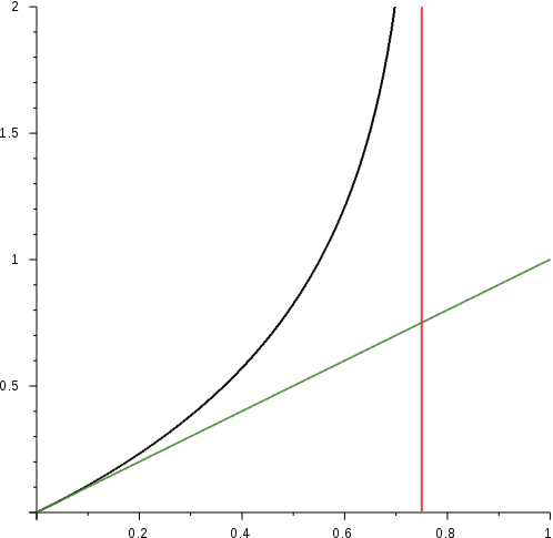
Black line denotes the curve, green is the trend line for small values of f while the red line denotes the asymptotic boundary.
Other Models
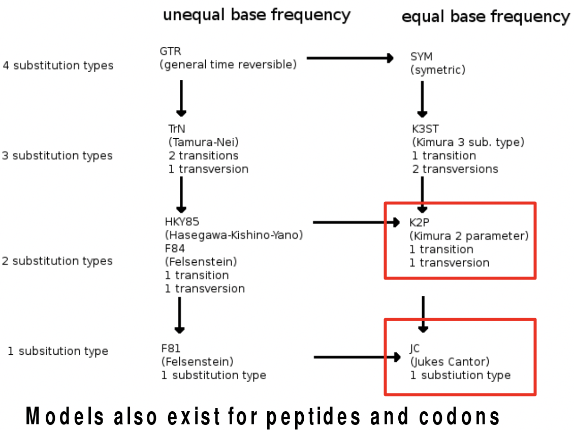
The Jukes Cantor model is the simplest model that gives us theoretically consistent additive distance model. However, it is a one-parameter model that assumes that the mutations from each base to a different base has the same chance. But, changes between AG or between TC are more likely than changes across them. The first type of substitution is called transitions while the second type is called transversions. The Kimura model has two parameters which take this into account. There are also many other modifications of this distance model that takes into account the different rates of transitions and transversions etc. that are depicted below.
FAQ
Q: Can we use different parameters for different parts of the tree? To account for different mutation rates?
A: Its possible, it is a current area of research.
Distances to Trees
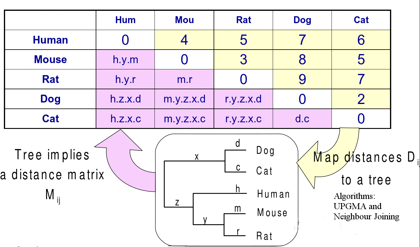
If we have a weighted phylogenetic tree, we can find the total weight (length) of the shortest path between a pair of leaves by summing up the individual branch lengths in the path. Considering all such pairs of leaves, we have a distance matrix representing the data. In distance based methods, the problem is to reconstruct the tree given this distance matrix.
Commons license. For more information, see http://ocw.mit.edu/help/faq-fair-use/.
Figure 26.9: Mapping from a tree to a distance matrix and vice versa
FAQ
Q: In Figure 27.9 The m and r sequence divergence metrics can have some overlap so distance be- tween mouse and rat is not simply m+r. Wouldn’t that only be the case if there was no overlap?
A: If you model evolution correctly, then you would get evolutionary distance. It’s an inequality rather than an equality and we agree that you can’t exactly infer that the given distance is the precise distance. Therefore, the sequences’ distance between mouse and rat is probably less than m + r because of overlap, convergent evolution, and transversions.
However, note that there is not a one-to-one correspondence between a distance matrix and a weighted tree. Each tree does correspond to one distance matrix, but the opposite is not always true. A distance matrix has to satisfy additional properties in order to correspond to some weighted tree. In fact, there are two models that assume special constraints on the distance matrix:
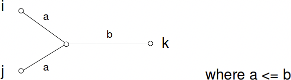
Ultrametric: For all triplets (a, b, c) of leaves, two pairs among them have equal distance, and the third distance is smaller; i.e. the triplet can be labelled i, j, k such that
\[d_{i j} \leq d_{i k}=d_{j k}\nonumber\]
Conceptually this is because the two leaves that are more closely related (say i,j) have diverged from the thrid (k) at exactly the same time. and the time separation from the third should be equal, whereas the separation between themselves should be smaller.
Additive: Additive distance matrices satisfy the property that all quartet of leaves can be labelled i, j, k, l such that
\[d_{i j}+d_{k l} \leq d_{i k}+d_{j l}=d_{i l}+d_{j k}\nonumber\]
This is in fact true for all positive-weight trees. For any 4 leaves in a tree, there can be exactly one topology, i.e.
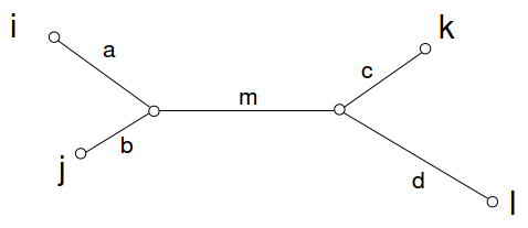
Then the above condition is term by term equivalent to
\[(a+b)+(c+d) \leq(a+m+c)+(b+m+d)=(a+m+d)+(b+m+c)\nonumber\].
This equality corresponds to all pairwise distances that are possible from traversing this tree.
These types of redundant equalities must occur while mapping a tree to a distance matrix, because a tree of n nodes has n 1 parameters, one for each branch length, while a distance matrix has n2 parameters. Hence, a tree is essentially a lower dimensional projection of a higher dimensional space. A corollary of this observation is that not all distance matrices have a corresponding tree, but all trees map to unique distance matrices.
However, real datasets do not exactly satisfy either ultrameric or additive constraints. This can be due to noise (when our parameters for our evolutionary models are not precise), stochasticity and randomness (due to small samples), fluctuations, different rates of mutations, gene conversions and horizontal transfer. Because of this, we need tree-building algorithms that are able to handle noisy distance matrices.
Next, two algorithms that directly rely on these assumptions for tree reconstruction will be discussed.
UPGMA - Unweighted Pair Group Method with Arithmetic Mean
This is exactly same as the method of Hierarchical clustering discussed in Lecture 13, Gene Expression Clustering. It forms clusters step by step, from closely related nodes to ones that are further separated. A branching node is formed for each successive level. The algorithm can be described properly by the following steps:
Initialization:
1. Define one leaf i per sequence xi.
2. Place each leaf i at height 0.
3. Define Clusters Ci each having one leaf i.
Iteration:
- Find the pairwise distances dij between each pairs of clusters Ci,Cj by taking the arithmetic mean of the distances between their member sequences.
- Find two clusters Ci,Cj such that dij is minimized.
- Let Ck = \(C_{i} \cup C_{j}\).
- Define node k as parent of nodes i, j and
place it at height dij/2 above i,j.
- Delete Ci,Cj.
Termination: When two clusters Ci, Cj remain, place the root at height dij/2 as parent of the nodes i, j
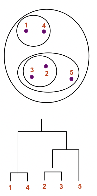
Ultrametrification of non-ultrametric trees
If a tree does not satisfy ultrametric conditions, we can attempt to find a set of alterations to an nxn symmetric distance matrix that will make it ultrametric. This can be accomplished by constructing a completely connected graph with weights given by the original distance matrix, finding a minimum spanning tree (MST) of this graph, and then building a new distance matrix with elements D(i,j) given by the largest weight on the unique path in the MST from i to j. A spanning tree of the fully connected graph simply identifies a subset of edges that connects all nodes without creating any cycles, and a minimum spanning tree is a spanning tree that minimizes the total sum of edge weights. An MST can be found using ie Prims algorithm, and then used to correct a non-ultrametric tree.
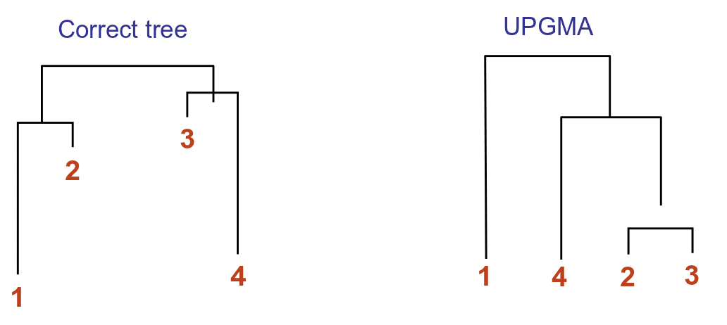
Weaknesses of UPGMA
Although this method is guaranteed to find the correct tree if the distance matrix obeys the ultrameric property, it turns out to be a inaccurate algorithm in practice. Apart from lack of robustness, it suffers from the molecular clock assumption that the mutation rate over time is constant for all species. However, this is not true as certain species such as rat and mice evolve much faster than others. Such differences in mutation rate can lead to long branch attraction; nodes sharing a lower mutation rate but found in distinct lineages may be merged, leaving those nodes with higher mutation rates (long branches) to appear together in the tree. The following figure illustrates an example where UPGMA fails:
Neighbor Joining
The neighbor joining method is guaranteed to produce the correct tree if the distance matrix satisfies the additive property. It may also produce a good tree when there is some noise in the data. The algorithm is described below:
Finding the neighboring leaves: Let
\[D_{i j}=d_{i j}-\left(r_{i}+r_{j}\right) \text { where } r_{a}=\frac{1}{n-2} \sum_{k} d_{a k}, a \in\{i, j\}\nonumber\]
Here n is the number of nodes in the tree; hence, ri is the average distance of a node to the other nodes. It can be proved that the above modification ensures that Dij is minimal only if i, j are neighbors. (A proof can be found in page 189 of Durbin’s book).
Initialization: Define T to be the set of leaf nodes, one per sequence. Let L = T
Iteration:
1. Pick i, j such that Dij is minimized.
2. Define a new node k,and set \[d_{k m}=\frac{1}{2}\left(d_{i m}+d_{j m} d_{i j}\right) \forall m \in L\nonumber\]
3. Add k to T, with edges of lengths \[d_{i k}=\frac{1}{2}\left(d_{i j}+r_{i} r_{j}\right)\nonumber\]
4. Remove i, j from L
5. Add k to L
Termination: When L consists of two nodes i,j, and the edge between them of length dij, add the root node as parent of i and j.
Summary of Distance Methods Pros and Cons
The methods described above have been shown to capture many interesting features of phylogenetic relationships, and are typically very fast in the algorithmic sense. However, some information is certainly lost in the distance matrix, and typically only a single tree is proposed. Serious errors, such as long branch attraction, can be made when basic assumptions about mutation rate etc. are violated. Finally, distance methods make no inference about the history of a particular site, and thus do not make suggestions about the ancestral state of a sequence.